Efficient Jointed Rock Slope Analysis using XFEM
An overview of the application of XFEM in jointed rock slopes for discontinuities
Introduction: Modeling jointed rock slopes is one of the more challenging problems in rock mechanics. The position and strength of the joints have significant impacts on the stability of the domain. The finite element method is one of the widely used numerical techniques for modeling jointed rock mass, where both joint and intact rock would be modeled separately.
However, the primary challenge of this technique is defining the mesh with joints in complex geometries. To overcome this limitation, the extended finite element method (XFEM) is introduced to identify the discontinuities individually, where the discretization is independent of joints.
This paper highlights the application of XFEM in jointed rock slopes with discontinuities and presents a mathematical framework for XFEM that can capture the effect of intersecting joints accurately.
Mathematical Formulations Explained
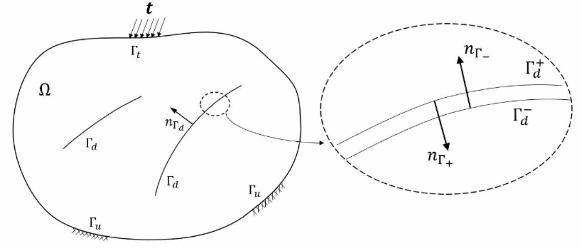
In this segment, the equation for a non-linear rock mass in 2D is reviewed. The domain Ω contains discontinuities with the boundary of Γ𝑑, under the external traction t applied on Γ𝑡 and internal body force b and prescribed displacements imposed on Γ𝑢.
A set of equations that are essential to describe the domain are the equilibrium equation and constitutive laws for the rock mass and the joint.
The equilibrium can be written as: 𝑑iv (𝝈) + 𝒃 = 0

Here, ⟦𝜹𝒖⟧ defines the jump of 𝜹𝒖 on both sides of the joints.
Discretization with XFEM
The discretization of the weak form equation (1) in space with the extended finite element method is discussed in this section. This method shows that nodes are enriched based on the type of discontinuity. The Heavside function (H(x)) is used here to capture the discontinuity in the domain, +1 on one side of the discontinuity, and -1 is used on the other side. Thus, if defines the displacement in the domain, it can be approximated by
(2)
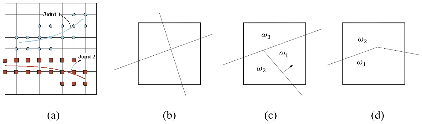
The approximation explained in equation (2) is accurate when joints are not crossing each other. Additional enrichment is required in this case, which is imposed using junction function As a result, if outlines all nodes whose support contains crossing joints, the approximation (2) can be revised as:
(3)

Here, ŭi is the additional unknown of the ith node due to assigning the junction function enrichment. Depending on the condition of crossing joints, three different forms of junction function are showcased.
Approximating the displacement in equation (3), the equilibrium equation interpreted in (1) can be written in the matrix form as follows:
(4)

B is a matrix containing the derivative of shape functions, and N is the shape functions in a vector form – including basic shape functions for all nodes and the enhanced shape functions for the enriched nodes.
Examples of Numerical Models
Two numerical examples of jointed rock slopes are solved using the XFEM technique and the results are compared by the explicit joint method.
Slope with Voronoi joint network
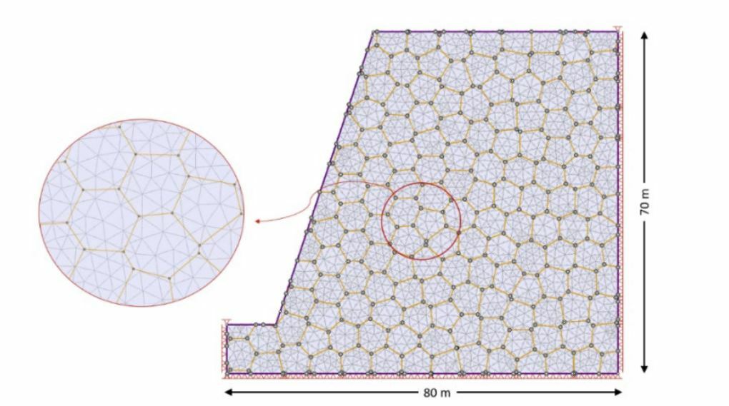
In this example, a jointed rock slope is examined to ensure stability. The geometry of the slope is shown in Fig 4. RS2’s Voronoi joint network is assigned to the slope where the dimension of the slope is 80mx70m and the slope angle is 72 degrees. It can be seen in Fig 4. that the mesh is independent of the joint network with the use of the XFEM approach.
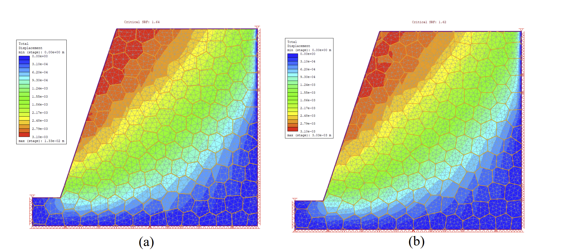
The shear strength reduction analysis is run to calculate the slope’s stability and the results are compared to the explicit joint method. Through this technique, the strength properties of the failure criterion (i.e. cohesion and friction angle) would reduce by a factor until the convergence cannot be met for the slope simulation. In this model, the SRF for the XFEM approach is calculated to be 1.64, whereas, for the explicit method, 1.62 is obtained. The total displacement contour for both models is outlined before the failure (SRF = 1.6).
Slope Excavation
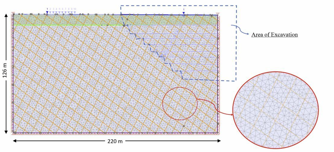
The excavation of the jointed rock slope is studied, and the geometry is shown in Fig 6. Where two sets of parallel joints are assigned to the rock that are intersecting each other. The rock slope is excavated in 10 stages – The water table is at the ground surface at the initial state & throughout the excavation, it is lowered by dewatering at each stage.
The analysis results from the traditional explicit joint method were then compared with the results obtained using the XFEM approach.
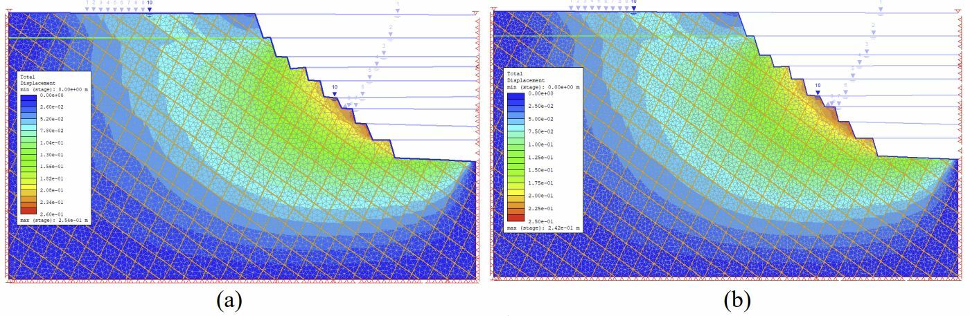
Figure 7 shows the total displacement comparison at the last stage of excavation between the XFEM and explicit joint methods. The results show a very similar pattern captured in the models above.
Final thoughts
This study illustrates the application of the XFEM method for general cases where joints are intersecting each other. It was shown that this method is completely mesh-independent and the joints can be placed anywhere in the model. In comparison to the joint network approach, XFEM can reduce the computation cost & time in solving problems with larger mesh sizes as the joints in XFEM are mesh independent.