Can Machine Learning Accelerate 3D Finite Element Modelling?
There are few certainties in geotechnical engineering, however, one thing that’s certain is “bad input data will produce bad results.” This statement highlights the importance of identifying or estimating representative material parameters in order to accurately evaluate ground behaviour. However, the complexity of geological materials can limit precise predictions and often require sensitivity analysis. This can be a time-consuming process, particularly when there is high uncertainty in material strengths.
How can we leverage Machine Learning?
Machine Learning (ML) algorithms can have many uses; rapid prediction, solving inverse problems, and anomaly detection to name a few. This paper applies ML to 3D finite element (FE) modelling using RS3 to derive material strengths for an open pit mine where the potential for structurally-controlled failure, along three intersecting structures, was identified. ML was integrated to identify feature importance (i.e. the most critical material properties in the model) and their critical strength. ML significantly reduced the manual requirement to vary material properties, recompute and assess model validity.
Case Study
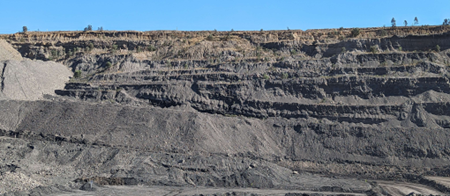
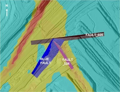
This paper examines a section of an open pit coal mine (Figure 1) where the stability was largely driven by three intersecting sub-vertical faults, and a basal sub-horizontal shear plane (Figure 2). Fault dip ranged from on average 60 to 81 degrees, and the basal shear plane dip, along top of coal, ranged from 5 to 15 degrees (Figure 2).
3D Finite-Element Model in RS3
A 3D FE model of the slope was constructed in RS3, recognizing the failure mechanism would be most appropriately modelling in three dimensions based on the intersections of modelled fault structures. Assuming slope stability in this section of the pit would primarily be structurally-controlled, the intact rock materials intersected in the slope were set as elastic to speed up computation time. The constructed 3D model extended approximately 550 m laterally, with a maximum 105 m in height. Bench scale slope angles ranged between 48 and 65 degrees.
Application of ML for Back-Analysis
Figure 3 summarizes the applied ML methodology. To start, a base RS3 model was constructed. A Python function was then created to duplicate the baseline FE model and adjust defect (fault and shear) properties based on initial estimated ranges (Table 1). In this case a uniform distribution was applied as ML models perform better when trained on evenly distributed data. Further a uniform distribution gives equal chance of the range of properties being applied to the models. A total of 30 RS3 models were computed with varying defect properties.
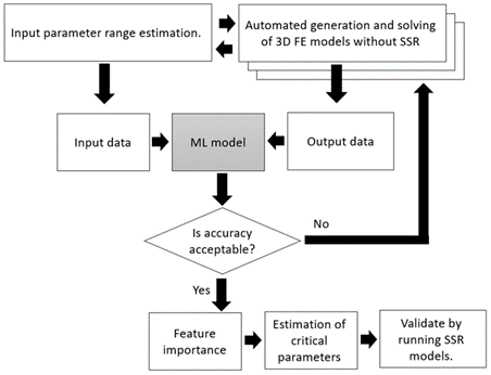
Table 1 - Estimated ranges of joint properties
Input Parameter |
Unit |
Mean Value | Range |
Normal stiffness |
MPa |
500 | ±50% |
Friction angle |
Degrees |
8 | ±50% |
Cohesion |
kPa |
10 | ±50% |
The 30 models were then split into training
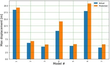
and test groups, and a Python ML script applied to assess acceptability of the models based on random forest-regression and random forest-classification algorithms. Acceptability criteria included the termination of a computation once the model performance was deemed satisfactory, allowing efficient computation of multiple models. An example of training versus test results is provided in Figure 4.
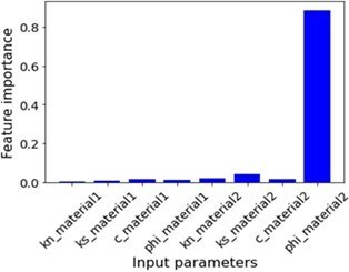
Feature importance was determined from random forest analysis. The results are displayed in Figure 5, concluding across all models that the sub-vertical faults’ friction angle to be the most impactful parameter on results. This finding allowed the subsequent modeling using shear strength reduction (SSR) calculations to focus solely on the calibration of the faults’ friction angle.
The results of convergence analysis were also queried to define the range of friction angle to run in SSR analysis. Figure 6 displays model displacement and convergence results at varying friction angles. Non-converging models were assumed to indicate slope failure, based on displacement criteria. From these results friction angles starting at 7 degrees (i.e. indicative of the boundary between non-converging and converging models) was entered into SSR models to identify the critical friction angle that would result in a strength reduction factor (SRF) of 1. In SSR models all other material parameters were kept constant.
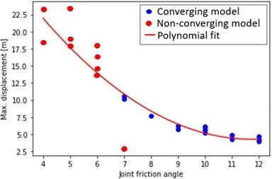
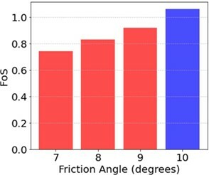
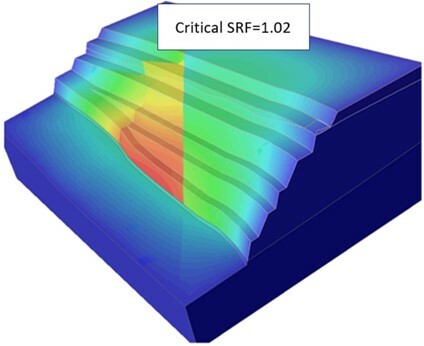
Figure 7 graphically summarizes the SRF results, indicating the critical fault friction angle for an SRF of 1 is between 9 and 10 degrees. Figure 8 displays the total displacement contours of the scenario where a friction angle of 10 degrees was applied to the SSR model, which resulted in a critical SRF of 1.02.
Key Takeaways
- Python functions were used to automate model creation, accelerate modification of input parameters and evaluate the acceptability of ML model results
- A small set of 30 models exhibited reasonable performance which demonstrates the potential of ML even for computationally demanding FE models.
- Calibration was achieved efficiently with minimal user intervention.
- In this case, the critical strength parameter identified (i.e. fault friction angle between 9 and 10 degrees) can be used by the geotechnical engineer to reconcile if this friction angle is representative of historical slope conditions, previous back analysis findings and/or available laboratory data. Then make determinations if slope instability is likely (or unlikely), and implement any subsequent design modifications to manage risk accordingly.
Could Machine Learning and Artificial Intelligence replace geotechnical engineers in the future?
We say it is highly unlikely. This study instead demonstrates how ML can be applied to execute specific geotechnical tasks more efficiently.
Where geotechnical engineering problems are generally unique due to varying natural ground conditions, each new model typically requires its own set of assumptions and simplifications, meaning there will always be the need for geotechnical professionals (real people) to make those explicit deductions.
However, we do believe the use of ML will integrate into the daily routine of geotechnical engineers more frequently in order to accelerate analysis, assist with calibration, and reduce the amount of manual work required.
Reference: You can read the full paper using this link: https://www.mdpi.com/2673-7094...