Analysis of Direct Shear Lab Data

1.0 Introduction

This tutorial will examine the fitting Mohr-Coulomb strength models to direct shear stress data (measured in psf units) for a soil.

Topics covered in this tutorial:

Finished Product:

The finished product of this tutorial can be found in the Tutorial 5.rsdata data file. All tutorial files installed with RSData can be accessed by selecting File > Recent Folders > Tutorials Folder from the RSData main menu.

2.0 Creating model

1. Open RSData.
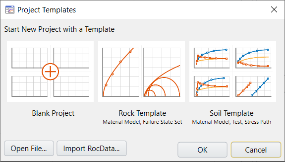
2. Select Blank Project for Project template and click OK.

3.0 Project Settings

We will define the units first.

1. Select Project Settings
2. Select Units = Imperial, stress as psf



>
3. Click OK.

Note: A warning message will appear when you change the units.



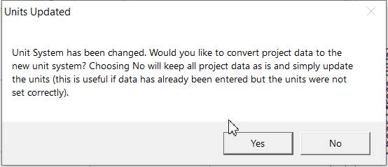
4. Click Yes. Since no new data was input, choosing Yes will not affect your results.

4.0 Material and Material Models

When you open a Blank template, a material is automatically created and added to the Visibility Tree on the left side of the screen.

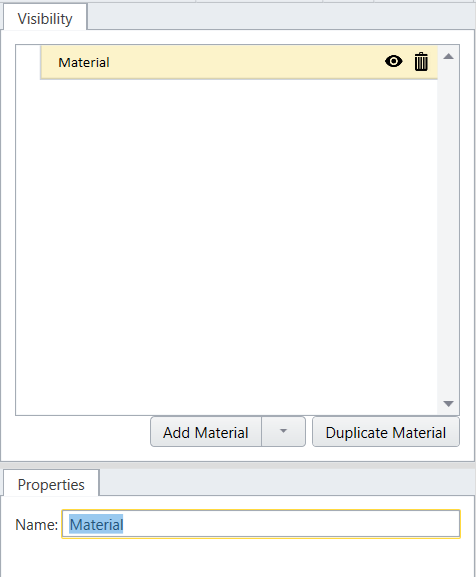
1. In the Visibility Tree, click on the Material.
2. Use the properties pane below to rename the new material to “Soil.”
3. Select Apply Material Models in the toolbar.
4. A dialog will appear. Assign the default material model “Material Model 1” to “Soil” as shown below:



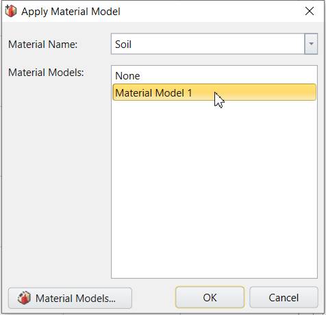
5. Click OK to save and close the dialog.

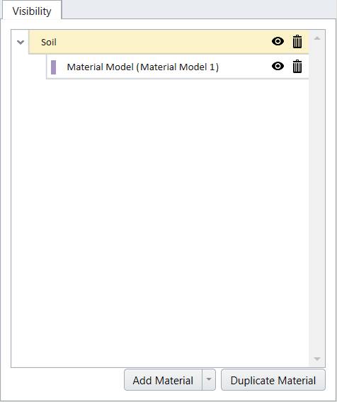
Now Material Model 1 has been applied to the Soil material.

5.0 Failure State

We will input the Direct Shear data points into the failure state.

1. Select Define Failure States in the toolbar.
2. In the properties section, define Failure State 1 as follows.
3. Select Test Type = Direct Shear Test.
4. Enter the following direct shear data points in the data grid:

	SigmaN (psf)	Tau
0	1	8.2
1	2	7.6
2	3	8.4
3	4	10.1
4	5	9.5
5	6	11.2
6	7	12.3
7	8	12.2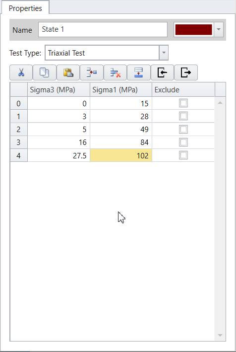



5. Click OK to save and close the dialog.
6. Select Apply Failure States.
7. In the Add Failure States dialog, apply State 1 to Soil as shown below:



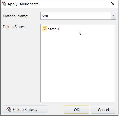
8. Click OK to save and close the dialog.

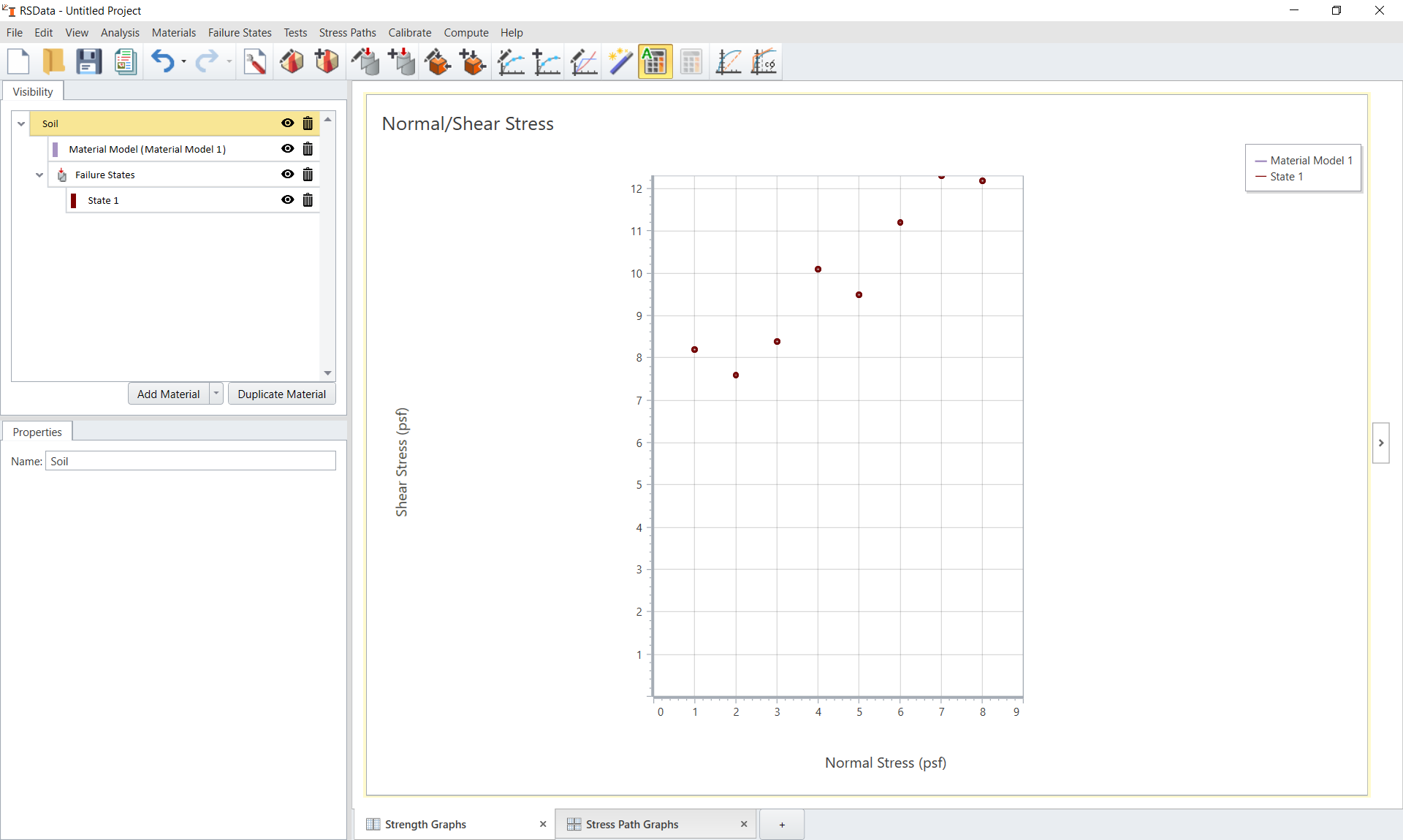
We are mainly focused on Normal vs. Shear Stress plot in this model. Double click on the Normal vs. Shear Stress plot. Direct Shear data points are drawn as data points as follows:

6.0 Calibration– Generalized Hoek-Brown

The next step is to curve fit/calibrate the field data set and find the best fit failure envelopes with the Mohr Coulomb method.

1. Under the Visibility Tree, right click on the Soil template, and select Apply Calibration.



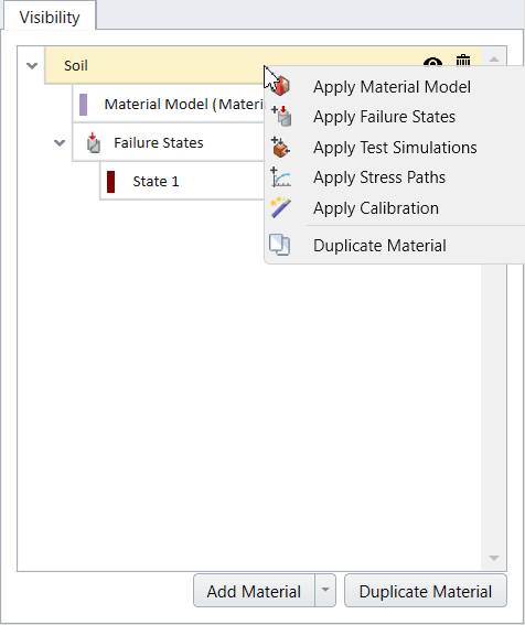
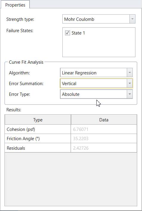
2. Select the added Calibration set under Soil. In the properties section below, enter the following:

• Strength type = Mohr Coulomb
• Algorithm = Linear Regression
• Error Summation = Vertical
• Error Type = Absolute

The calibration properties section should look as follows:

7.0 Results

By default the Auto Compute is selected and the result will be updated. The user has control to toggle the Auto Compute on and off. If Auto Compute is toggled off, be sure to select Compute to compute the calibration.

The numerical calibration results are summarized in the table under calibration properties section as shown below.

The calculated parameters are:

• Cohesion (kPa) = 6.76
• Friction Angle (⁰) = 35.22
• Residuals = 2.43

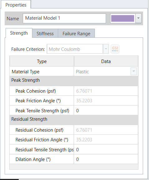
The calibration results will also be updated to the material model. We can check by selecting Material Mode (Material Model 1) in the Visibility Tree, and viewing the properties pane below. The Strength parameters and Failure Range parameters are recalculated.

7.1 GRAPHICAL CALIBRATION RESULTS

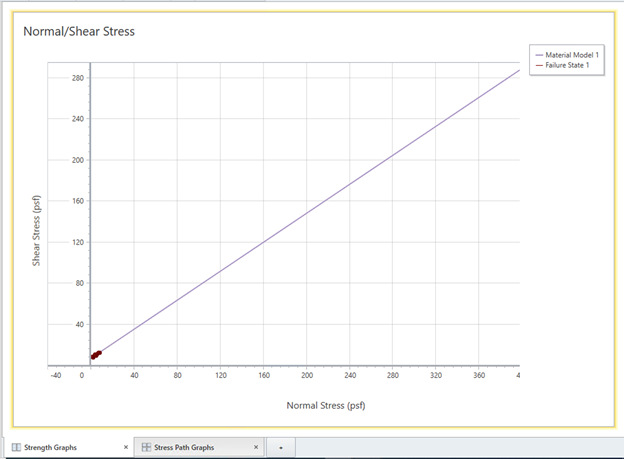
Failure envelopes also updated on the Normal vs. Shear Stress plot as displayed below.

To better view the failure state area, we need to adjust the failure envelope range.

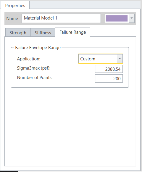
1. Select Material Model (Material Model 1) under the Visibility tree.
2. In the Properties section below, select the Failure Range tab and enter:

• Application = Custom
• Sigma3max (psf) = 30

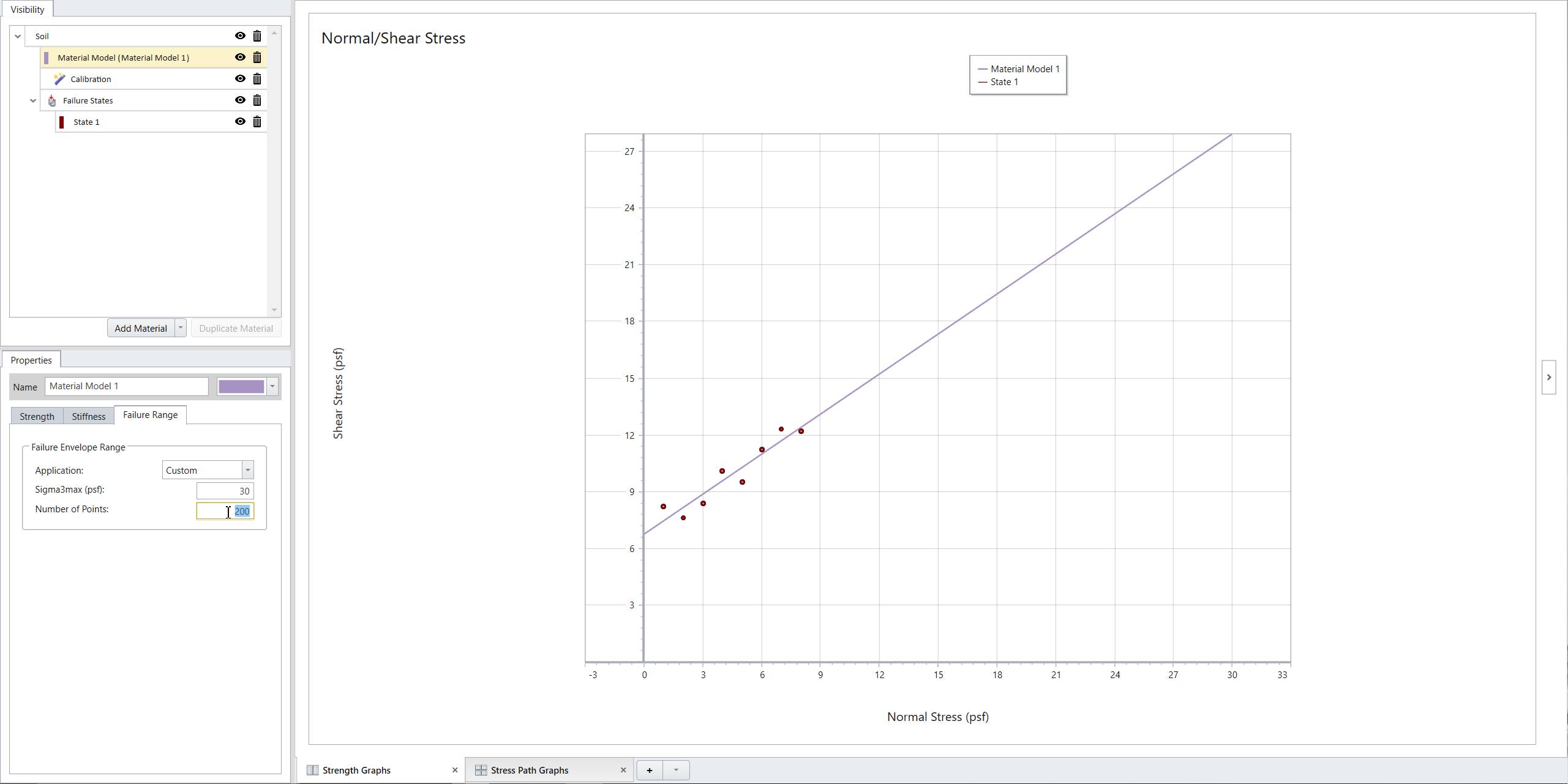
The calibrated failure envelope is depicted in a purple line. It can be observed that the line is fitting the direct shear dataset well.

This concludes the tutorial on fitting the Mohr-Coulomb strength model to a direct shear dataset.