By Ahmed Mufty, Ph.D., P.Eng.

Introduction

Traditionally, the settlement of a clay layer may be estimated based on results of one-dimensional consolidation tests carried out on samples obtained from the ground. The change in void ratio with effective stress is plotted in a semi-logarithmic graph where the vertical effective stress forms the horizontal axis in the logarithmic scale while that void ratio forms the vertical axis. Later, the graph is idealized in the form shown in Figure 1.

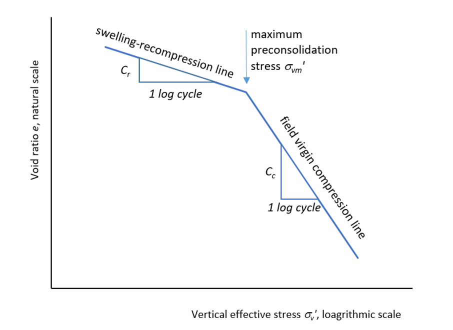
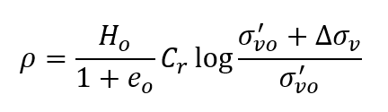
In a normally consolidated soil where the preconsolidation stress is equal to the existing effective stress (overburden pressure in naturally deposited soils), the settlement is calculated as:

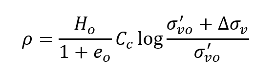
In this case, the overconsolidation ratio OCR or σ'_vm/σ'_vo is equal to one and the stress is moving along the virgin compression line and C_c is the compression index. H_o is the thickness of the clay layer and e_o is the initial existing void ratio corresponding to the existing initial effective stress σ'_vo. When OCR is greater than unity, and the existing effective stress is less than the maximum preconsolidation stress the settlement is calculated along the swelling line and if the additional stress ∆σ_v pushes the stress above σ'_vm then another part is added to the settlement as the stress point will be again on the virgin compression line.

If OCR>1 and the final effective stress σ'_vf'=σ'_vo'+∆σ_v is still less than σ'_vm then the settlement is calculated as:

If the final stress σ'_vf passes σ'_vm then the settlement is calculated as:

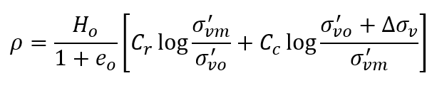
The soil property C_r is called the swelling or recompression index.

Geotechnical engineers are used to averaging the properties through the clay layer and use one equation for the hole thickness of the layer to calculate the settlement based on the effective stresses at the middle of the layer depth.

How does Settle3 work?

Settle3 subdivides the clay layer into subdivisions to get more accurate results. The soil properties may vary with depth and hence, the user can use datum dependency tab in soil properties dialogue box. See Figure 2.

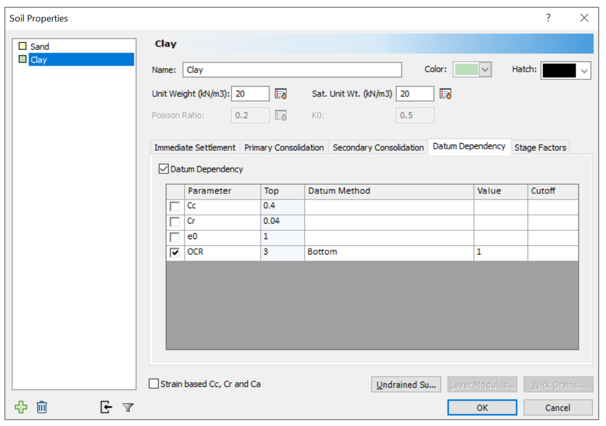
The most two important parameters that are encountered to be variable with depth are the void ratio and the overconsolidation ratio (in Settle3 overconsolidation may be represented also by OCM, overconsolidation margin, or by the preconsolidation stress directly). The effect of varying these parameters will be discussed later.

The software calculates settlements at query points (or lines) chosen by the user. The query point properties include the number of subdivisions of each layer the user wants to imply. See Figure 3. The dialogue box includes the query point name, its display settings, and the method used for subdividing the layers. The default is Automatic, but the user may change it to equal thickness sublayers or force the program to specific numbers of subdivisions in each layer.

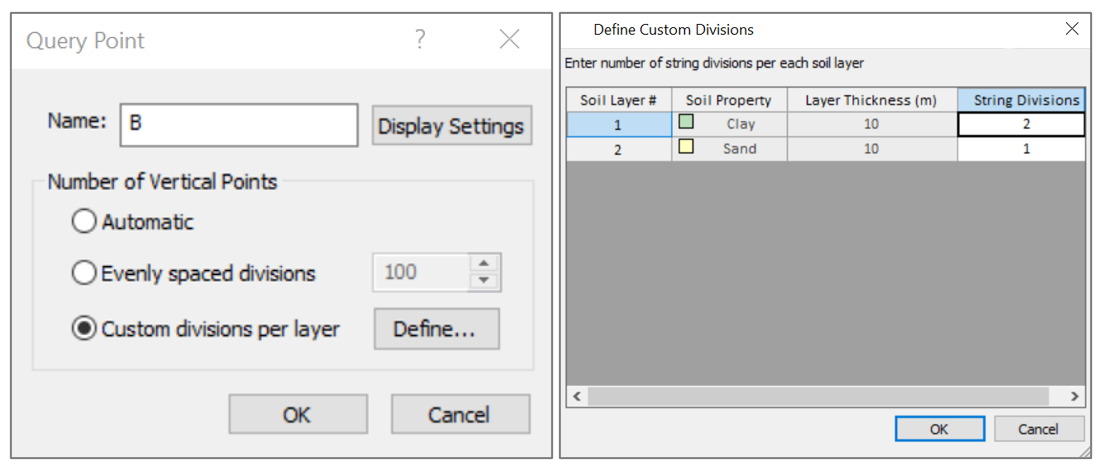
Any number above 1 will divide the layer into sublayers. So, the settlement of the layer will be the accumulation of settlement values of the sublayers:

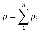
where i is the number of the sublayer within the layer that is divided into n divisions.

Hence, for each layer, the program calculates different thickness, initial and final effective stresses (depending on the method adopted by the user for stress distribution), the initial void ratio, preconsolidation stress (from the overconsolidation input in soil properties), and/or any other properties that vary with depth such as the compression index, swelling index, etc.

This subdivision will lead to a different result for the total settlement because of the nonlinear nature of the logarithmic part in the equations and the difference will increase with the complication of stress distribution and variation of soil properties with depth. The effect of the difference of subdivision will be less if the method chosen for the settlement calculation is the linear m_v method and the difference vanishes if the stress is distributed through the depth uniformly or linearly. Of course, the less the layer thickness compared to loading area the less is the difference between calculations based on one layer with average properties and calculation of settlement based on subdivisions with varying soil properties.

On the other hand, a nonlinear method with a variation of soil properties with depth and nonlinear stress distribution will yield greater differences between single whole layer computations and sublayers computations.

Examples and Discussion

In order to demonstrate the effect of subdividing a clay layer on the resulting calculated settlement in Settle3, a model comprising of a uniform load of 100 kPa applied to a clay layer of 10m thickness is tested. The clay properties are chosen as follows:

Initial void ratio e_o 1.0

Compression index C_c 0.4

Recompression index C_r 0.04

Overconsolidation ratio OCR 1.0 (normally consolidated clay)

Saturated unit weight γ_sat 20 kN/m3

The properties are kept unchanged through the layer depth to lessen the variables and concentrate on the main issue of layer subdivision. The groundwater is taken at the ground surface and the unit weight of water is entered as 10 kN/m³ to ease the hand calculations.

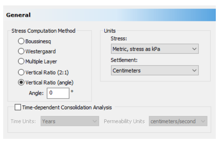
A load of 100 kPa is applied at the surface and over a large area 200mx200m and the load is uniformly transmitted through the depth using no stress distribution (zero angle for distribution in Settle3 “Project Settings” - General), see Figure 4. This keeps ∆σ_v unchanged through the depth.

Only primary settlement is checked and only in the clay layer. Six query points are added. Each query point is given different number for layer divisions using the query point property dialogue. The query points are for the following cases studied,

Point A is a whole layer choice, i.e. number of divisions= 1.

Point B, C, and D are for 2 divisions, 4 divisions, and 100 divisions respectively.

The last point F is chosen with automatic subdivision.

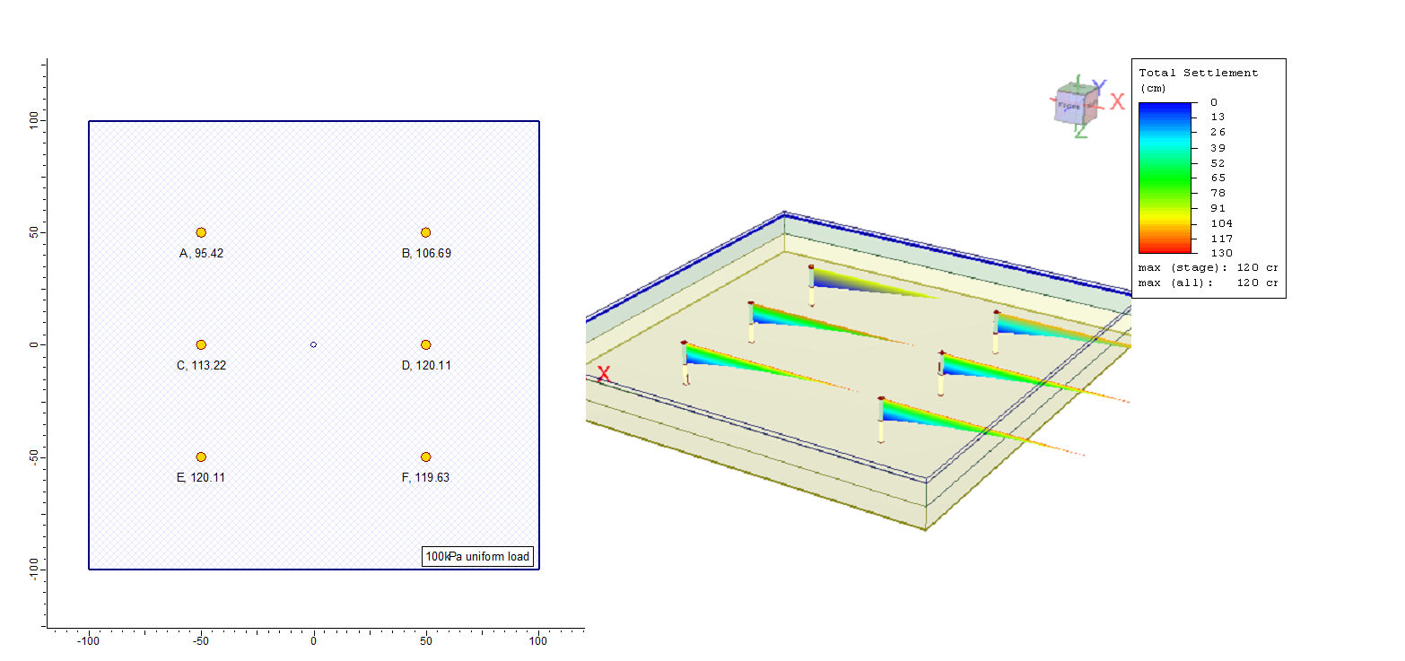
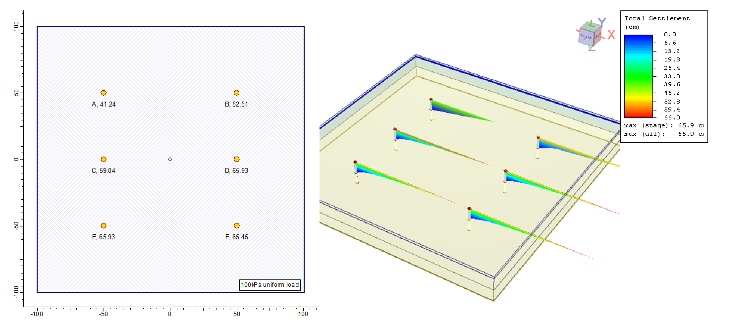
Figure 5 shows the plan and the 3D views of the model with calculated settlements displayed at the query points. It is clear that the settlement results are different except for points D and E where the number of divisions is forced to be 100 at each one. The clay layer is the green 10m thick layer at the ground surface and under the surface load directly. The settlement calculations are limited to the primary compression in the soil properties dialogue box, refer to tutorials of Settle3 at www.rocscience.com.

Hand calculation of settlement with average properties using the whole layer can be done easily as follows:

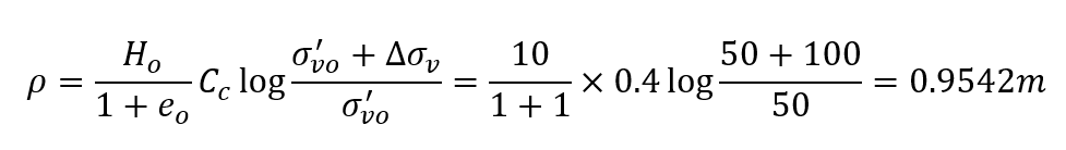
where the initial effective stress 50 kPa is calculated at mid-depth of the layer. The results are similar to point A where no divisions are applied.

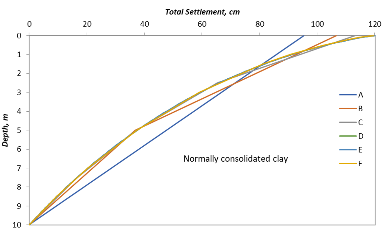
Comparing with other points, it can be seen that increasing the number of divisions increases the calculated settlement although the automatic divide gave a little bit less than the 100 divisions result. The settlement with depth is plotted for all the points in Figure 6.

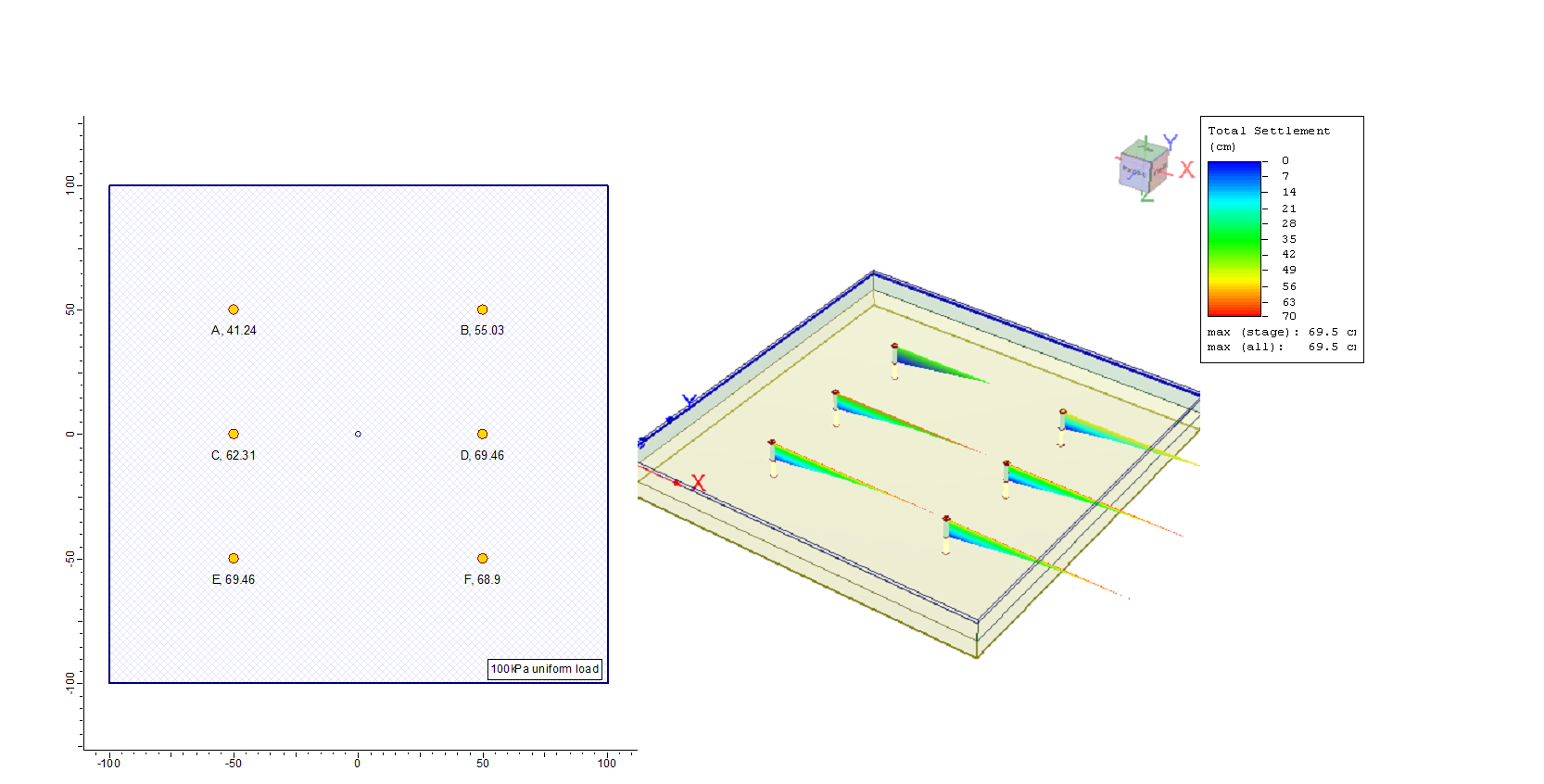
Another model with all the same as the previous model except that the clay is changed to an overconsolidated layer with constant OCR=2 with depth. Figure 7 and Figure 8 show the model and the settlement at the query points.

Calculating average layer settlement for overconsolidation ratio of 2, i.e. average σ'_vm=100 kPa, the final stress passes the maximum preconsolidation stress as it is 150 kPa, hence,

Note it is the same as the result of query point A.

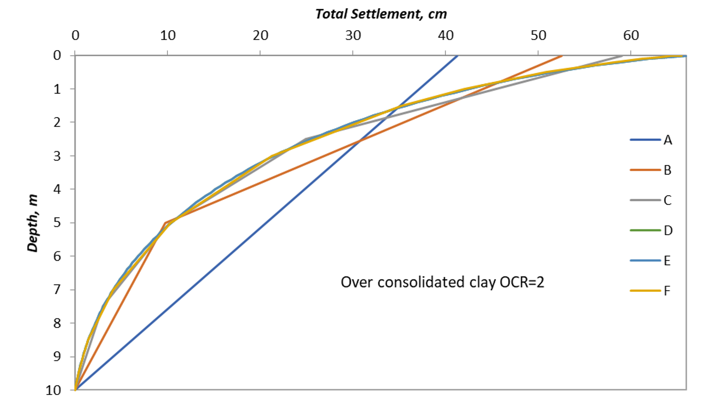
Similar to model 1, the increase in a number of divisions increased the estimated settlement except that in model 2 the settlement is less than model1 because of the overconsolidation.

A third model is presented as well, see Figure 9. In model 3, the overconsolidation ratio is varied with depth from 3 at the surface to 1 at the bottom of the layer. Using the average layer calculations, the settlement should be equal to model 2 as the average OCR in model 3 is equal to the constant OCR of model 2, compare points A, while the results of the other query points are different and that is because of calculating each subdivision based on its own OCR value varying with the depth of the subdivision. The results are plotted similarly to the other models in Figure 10.

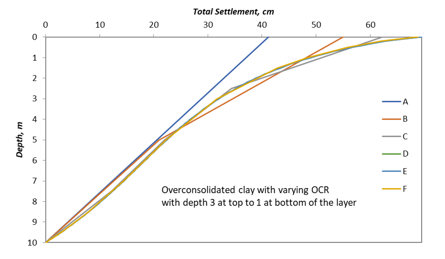
It can be depicted from the figures, that the effect of subdivisions on the result is greater in overconsolidated soil than in normally consolidated soil due to the intrusion of C_r, and it is even more obvious in the case of varying OCR with depth.

Effect of subdivision with linear soil properties

The same model is solved with the clay model changed from nonlinear to a linear one. In this case, a value for mv is chosen to be close to the average expected one as

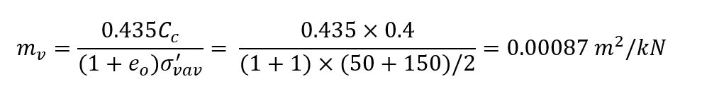
This value is used for the settlement calculation in Settle3 and all points regardless of the number of subdivisions gave the same result which is also equal to the average layer calculated one. That is

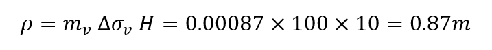
This makes clear that linear soil will not suffer any differences in settlement calculation due to subdivisions in the query points. Nevertheless, the result may be different than the nonlinear soil behavior even if the modulus is chosen very carefully.

Conclusions and Recommendations

The following points may be summarized from the discussion of the layer subdivision effects on settlement calculations of a clay layer in this article:

1. Subdividing a layer under nonlinear soil behavior or stress distribution will result in different values of settlement than using the traditional whole layer with average properties and stresses.
2. The difference will disappear in the case of linear soil properties and linear stress distribution.
3. The difference will decrease as the soil layer thickness is less compared to the loading area.
4. Subdivision is generally more conservative and yields higher settlement results.
5. It is recommended to increase the number of sublayers until settlement difference will be within an acceptable tolerance or at least to choose the automatic sublayer division in Settle3.
6. The engineer should not expect equal results from linear methods and nonlinear methods, and it is to his/her judgment what to adopt.
7. Increasing the nonlinearity of soil properties or stress distribution with depth yields more difference in settlement obtained from a different number of layer subdivisions.
8. The idea is general and may apply to all types of settlement and soil types.

Further reading

1. Lambe, T.W. and Whitman, R.V. (1969): Soil Mechanics, John Wiley and Sons. Chapters 8 and 12.
2. Settle3 Theory manuals, www.rocscience.com.

--

More from Rocscience