by Dr. Ian Williams

This article considers the feasibility of using Slide3 to help identify slope instability hazards associated with old coal tips in Wales.

Over the last few years, increased rainfall attributed to climate change has triggered landslides at several old coal tips in Wales. One of the first and most dramatic of these occurred at Tylorstown in February 2020 – see here.

In response to ensuing safety concerns, the Welsh and UK Governments set up a joint Coal Tip Safety Taskforce to assess the status of disused coal tips in Wales. Work is ongoing, but interim data published in October 2021, identifies a total of 2,456 coal tips in Wales with 327 being classified as representing a ‘higher potential risk’.

Gauging slope instability hazards at such a large number of sites presents a significant logistical challenge and, at present, appears to rely primarily on regular site inspections to identify signs of tip movement and the need for maintenance work. This approach raises the question of whether slope stability analyses are feasible as a rapid screening tool to enhance the understanding of potential slope instability hazards and help inform proactive decision-making.

In this context, this article considers whether three-dimensional limit equilibrium slope stability analyses using Slide3 have the potential to produce useful results for practical application to this class of problems. Since site-specific data is rarely available for old coal tip sites in Wales, the work has been based solely on public domain information and simplified/idealised models that can be built and analysed within a few hours.

It should be recognised that because the results presented are derived from highly idealised and simplified models they may not be wholly representative of actual field conditions.

Modelling methodology and information sources

To achieve the aforementioned objective, a simplified Slide3 model of an existing coal tip has been built and analysed. In recognition of the large number of tips identified by the Coal Tip Safety Taskforce and the very limited data generally available, a key objective was to build the model in a timely manner based solely on readily accessible public domain information. In this regard, two key simplifications have been to: (i) consider only slip surfaces contained wholly within the colliery discard; and (ii) ignore the underlying geology/hydrogeology.

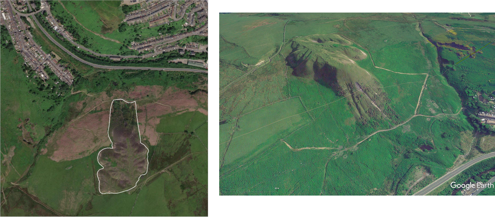
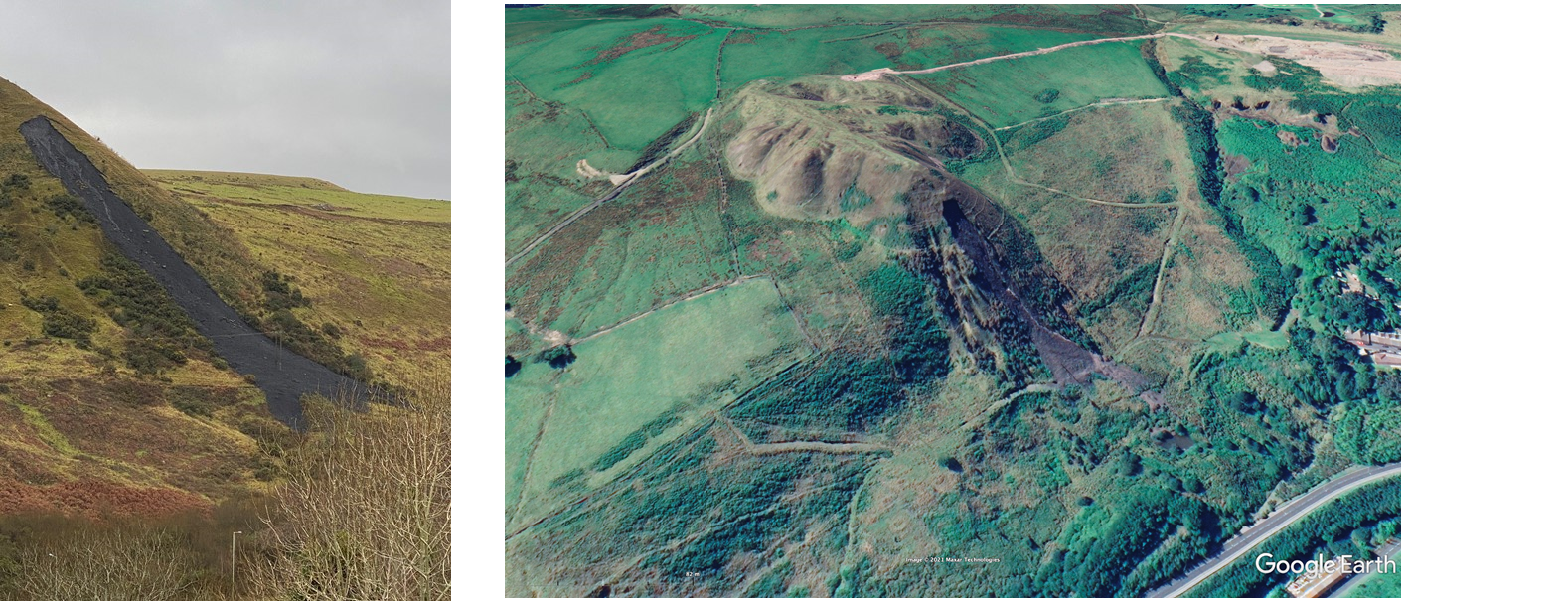
The coal tip selected for the study is the Wattstown Standard Tip in Rhondda Cynon Taff, South Wales (see Figure 1a).

The tip stands on a north-facing valley slope above the village of Wattstown and is estimated to cover a plan area of around 85,000 m², attain a maximum depth of around 40 m and accommodate around 1 million cubic metres of colliery discard.

The topography of the tip can be seen on Google Earth at WGS84 coordinates (51.629788°N, -3.423266°E). One of the available Google Earth images, dated July 2013, is presented in Figure 1b. This shows the irregular topography of the tip and several erosion gulleys on its north-facing slope. The substantial spoon-shaped depression at the top of the easternmost erosion gulley is strongly suggestive of a previous landslip at that location.

Public domain LiDAR terrain model data covering approximately 70% of Wales is freely available from the Natural Resources Wales composite dataset. The 1 m terrain model dataset obtained from this source has been used to represent the ground surface topography for the Slide3 model of the tip as shown in Figures 2 and 3.

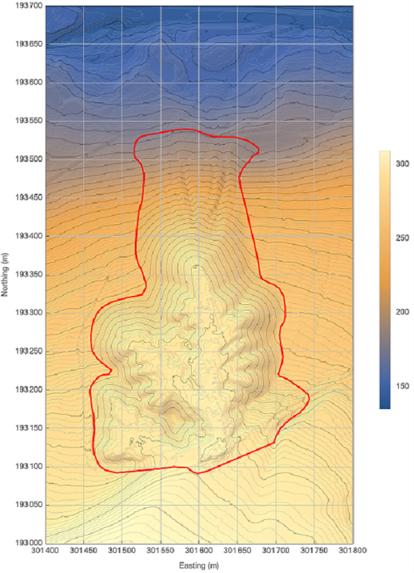
Based on these LiDAR data, the maximum slope angles of the tip’s perimeter slopes is around 36°. The highest, north-facing, section of slope falls by around 90 m from elevations of around 290 m AOD at the slope crest to around 180 m AOD at the toe.

During heavy rain on 18^th December 2020, a significant landslide is reported to have occurred on the tip’s north-facing slope. Photographs of the landslip are presented in Figure 5(a) and Figure 5(b). Based on these photographs, the landslip appears to have comprised relatively shallow rotational and/or translational movement on the upper slope initially with a resulting debris flow blanketing the lower slope.

The photographs also suggest that a curved tension crack may have developed to the west of the landslip’s exposed crown. Whilst appreciable ground displacement appears to be evident in this area, the movement did not evolve and contribute to the debris flow. It is therefore possible that the initial slip surface is considerably wider than might be inferred from the exposed colliery discard and debris flow alone.

Slide3 Modelling

The construction of the Slide3 model was a quick and simple process and is described in steps 1 to 5 below.

Step 1: Import the LiDAR terrain model data

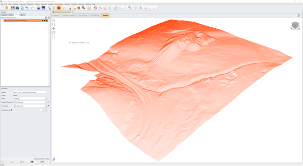
The ground surface model was derived from public domain LiDAR terrain model data downloaded in ESRI ASCII Grid format from the Natural Resources Wales composite dataset imported directly into Slide3 as a point cloud – see Figure 6.

Step 2: Triangulate the imported LiDAR data and define the model domain

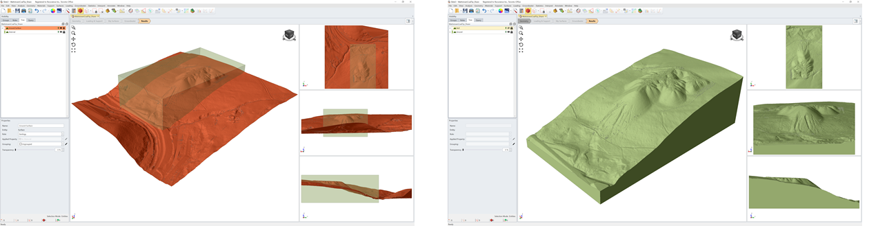
The imported LiDAR data was triangulated in Slide3 to form a surface (representing the ground surface) and an external box was created by specifying two diagonally opposite corner points to define the model domain as shown in Figures 7(a) and 7(b).

Step 3: Delineate the coal tip from the natural ground

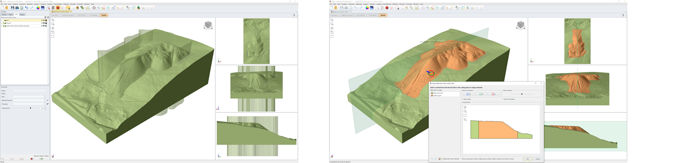
The proper separation of the coal tip from the underlying natural ground would require the original ground surface to be defined in the model. Since the estimation of this surface is relatively time-consuming, a simplified approach was adopted. The approach involved separating the coal tip region of the model in the vertical direction such that the tip extends to the base of the model domain. This was achieved quickly and easily by defining a 2D polyline around the tip perimeter in the horizontal plane and then extruding the polyline in the vertical direction so as to intercept the top and bottom surfaces of the model domain as shown in Figure 8 (a).

The two regions of the model delineated by the extruded polyline were then divided and material models were assigned to the region representing the colliery discard and to the region representing the natural ground. The resulting model is shown in Figure 8 (b).

Step 4: Define the geotechnical parameters

Site investigation data is unlikely to be available for many, if not most, of the old coal tips in Wales. For preliminary slope stability modelling, it will therefore often be necessary to rely on authoritative guidance and engineering judgement to estimate suitable shear strength criteria for the materials represented in computational models.

Empirically derived strength criteria for colliery discard are published in Reference 1. For coarse colliery discard in South Wales, Reference 1 states that the peak shear strength can be approximated by the following relationship:

t = 1.31 s' ^0.9  (1) 

in which t is the effective peak shear strength and s' is the effective stress normal to the plane of failure.

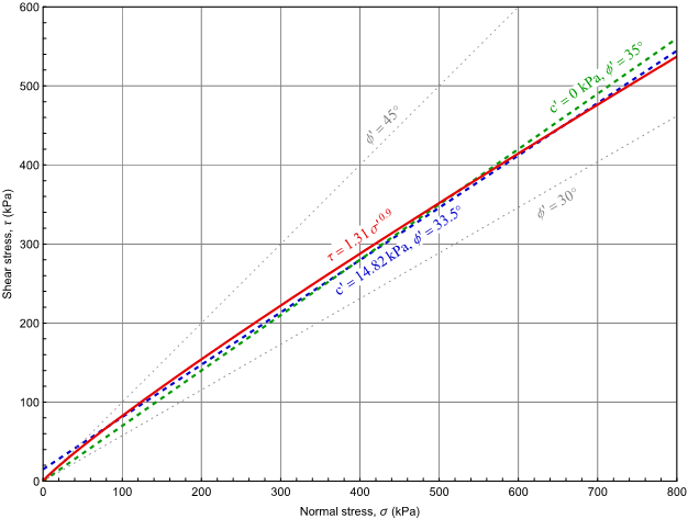
For comparison purposes, the linear Mohr-Coulomb shear strength envelopes for peak shear strength parameters c' = 14.82 kPa / f' = 33.5° and c' = 0 kPa / f' = 35.0° are also plotted on Figure 14. These Mohr-Coulomb parameters are taken from Reference 2 and are derived from the results of 49 consolidated-drained triaxial tests on samples from a colliery discard spoil heap in Yorkshire. The Mohr-Coulomb failure envelopes compare favourably with the curved failure envelope given by Equation 1: this provides some reassurance that Equation 1 is not an unreasonable estimator for the shear strength of the colliery discard.

For the analyses presented in this article, the shear strength of the colliery discard has therefore been represented by Equation 1. In Slide3, this was modelled using the Power Curve failure criterion with the parameters a = 1.31 and b = 0.9.

The unit weight of the colliery discard was taken as 18 kN/m³.

To ensure that all trial failure surfaces were contained wholly within the colliery discard, Slide3’s Infinite Strength failure criteria were assigned to the natural ground outside the tip perimeter. It was therefore not necessary to include the natural ground in the Slide3 model and it was represented only to provide context for the visualisations.

Step 5: Define the groundwater regime

The groundwater regime within the coal tip was the most challenging unknown in terms of its representation in a preliminary slope stability model. In considering the best way to represent possible groundwater conditions within the tip, various trials were undertaken, including:

• placing the groundwater table at some fixed depth below the ground surface;
• placing the groundwater table at some fixed depth above the estimated base of the tip; and

• placing the groundwater table at some elevation defined by a head of water as a fraction of the tip depth above the estimated tip base.

The results of these trials are not presented. However, none were deemed satisfactory for preliminary assessment purposes because: (i) they added significant complexity and time to the model building task; and (ii) they failed to produce critical slip surfaces that were a close match to the landslip that occurred in December 2020.

It was therefore decided to try using Slide3’s R_u coefficient to represent the pore pressure as a fraction of the vertical earth pressure at any given depth. Using this approach, setting R_u = 0 represents dry conditions within the tip. Whilst for colliery discard and water unit weights g_s = 18 kN/m³ and g_w = 9.81 kN/m³ respectively, setting R_u = g_w / g_s = 0.545 corresponds to fully saturated conditions with the groundwater table at the ground surface and hydrostatic groundwater pressures.

Using an R_u coefficient to represent groundwater pressures in a Slide3 model would not normally be promoted. However, for this case, it gave a critical slip surface that closely resembled field observations and had the advantage of being trivial to implement. In the context of simplified preliminary modelling where the true groundwater regime is in any event unknown, using Slide3’s R_u coefficient to represent pore pressures may therefore not be unreasonable.

Analysis and Results

The model described above was analysed for various values of the R_u coefficient and the results are summarised below. All results were computed using the GLE/Morgenstern-Price analysis method. Slide3’s automated Multi-Modal-Optimization (MMO) search method with Surface Altering Optimization was used to seek out the critical slip surfaces. The MMO search method is a relatively new addition to Slide3 and has the benefit of searching for multiple potentially critical slip surfaces rather than focusing on the single, most critical, surface.

Slide3 results for the tip in the dry condition, R_u = 0

In the first instance, the stability of the coal tip under dry conditions, without any pore water pressure effects, was considered. The Slide3 analysis identified the three potential slip surfaces shown in Figure 10. The global minimum factor of safety was 1.219 and is consistent with the stable condition of the tip prior to the landslip in December 2020.

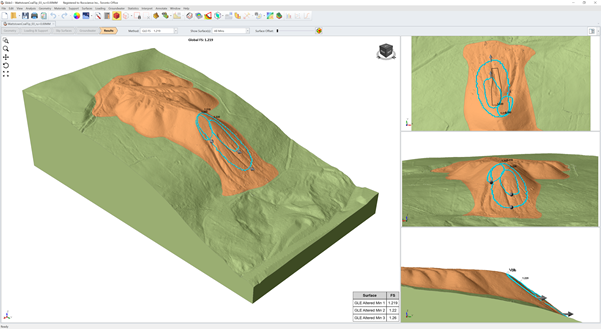
The factors of safety for all three critical slip surfaces are very similar. For the first two critical slip surfaces, the factors of safety differ by less than 0.1 % and are practically identical. The positions of the critical slip surfaces and geometries of the sliding masses are, however, very different. As can be seen from the characteristics given in Table 1, the maximum depth and volume of material for the most critical slip surface are considerably greater than those for the (marginally) second most critical slip surface. One implication of this observation is that in practice, either (or a combination) of these two slip surfaces could be the most critical.

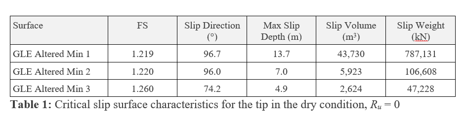
Figure 11 presents the surface safety map for the tip in dry condition. This shows that the most critical area of the tip is its north-facing slope where factors of safety generally range from around 1.2 to 1.5. Factors of safety then rise with increasing distance from the tip’s north-facing slope. The only exceptions are relatively small, localised areas on the tip’s western and eastern flanks where potential slip surfaces on the west and east boundary slopes buck the general trend.

Slide3 results for the tip with pore water pressure effects, R_u = 0.13

To introduce the effects of increased pore water pressures within the tip, a series of analyses were performed in which the R_u value of the colliery discard was incrementally increased until the global minimum factor of safety fell to just below unity. The critical slip surfaces shown in Figure 12 were thus obtained using an R_u value of 0.13 for which the global minimum factor of safety was 0.986.

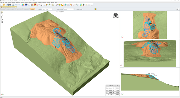
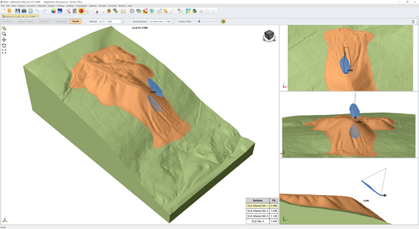
Figure 13 shows the most critical slip surface in isolation together with the approximate position of the actual slip surface as traced from Google Earth (see plane view in the top-right pane of Figure 13). The surface expression of the most critical slip surface is a very close match to the uppermost region of the actual slip surface. Referring to the possible curved tension crack to the west of the landslip’s exposed crown, the most critical slip surface shown in Figure 13 may be an even better match to the position of the actual slip surface whose traced position does not include the region of inferred region of lesser slope movement to the west of the exposed colliery discard.

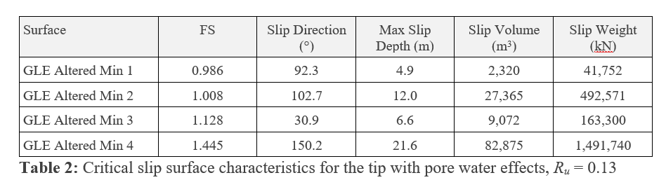
Again, whilst the factors of safety for the first two critical slip surfaces are quite similar, the positions of the slip surfaces and geometries of the sliding masses are very different. As can be seen from the characteristics given in Table 2, the maximum depth and volume of material for the most critical slip surface are considerably less than those for the second most critical slip surface. Although there is no quantitative field data against which the computed values given in Table 2 can be compared, the maximum depth of 4.9 m for the most critical slip surface does not appear to be grossly inconsistent with the photographs shown in Figure 5(a) and 5(b).

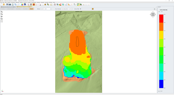
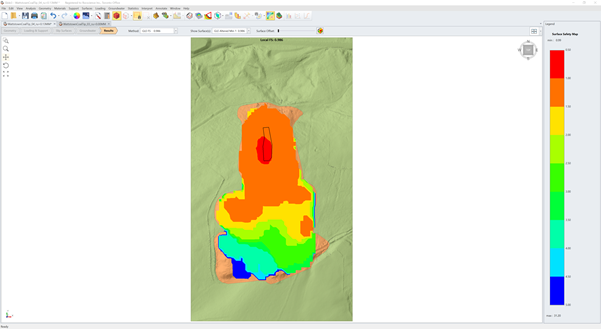
The close match between the most critical slip surface computed by Slide3 and the position of the actual slip surface is also apparent from the surface safety map presented in Figure 14.

Conclusions

Some conclusions arising from the work presented above can be summarised as follows.

1. Slide3 identified the origin of the landslip that occurred on the Wattstown Standard Tip with remarkable precision.
2. The results were achieved with very limited information and a highly idealised ground model.
   
3. By simplifying the Slide3 model, it was possible to set-up the model and run the analyses in less than half a day (circa 3 to 4 hours). This is an important consideration in the context of preliminary stability studies, especially if many sites need to be examined.
   
4. The simplifying assumption that the coal tip was not bottomed-out by natural ground such that the colliery discard extended to the base of the model domain was of little consequence in this case. This is because the critical slip surfaces were relatively shallow and, by inspection, did not extend significantly into the natural ground. This may not be the case for other topographies and would need to be considered on a case-by-case basis.
   
5. Modelling the effects of pore water pressure using an R_u coefficient was trivial to implement and, for this case, resulted in the surface expression of the most critical slip surface being a very close match to field observations.
   
6. The findings suggest that Slide3 has great potential for use as a rapid screening tool to help identify locations on old coal tips in South Wales where future landslips will most likely originate. Such information could help to inform proactive decision making regarding the need for more detailed investigation/assessment and/or targeted drainage, stabilisation or other maintenance works.
   
7. 3D slope stability analyses can be simpler and less time consuming than traditional 2D analyses. This is particularly true for irregular topographies where the locations(s) of the most critical slip surface(s) may not always be obvious and/or where there is a significant potential for landslips to occur at multiple locations. 3D analyses also have the potential to yield more reliable results.
   
8. Because the analyses presented in this article are based on an assumed shear strength for the colliery discard together with a highly simplified representation of an unknown groundwater regime, the computed factors of safety may not be fully representative of actual field conditions. To enhance confidence in the computed factors of safety, site-specific measures of the shear strength and unit weight for the colliery discard would be required together with an adequate understanding of the groundwater regime, including transient variations during a range of weather conditions. The underlying natural geology and hydrogeology, including possible impacts arising from the presence of old mine workings, may also need to be considered.

References

1. Handbook on the Design of Tips and Related Structures, prepared for the Department of the Environment by the Geoffrey Walton Practice, March 1991, London: HMSO.

2. The geotechnical characteristics of a spoil heap at Yorkshire Main Colliery, R. K. Taylor and D. A. Spears, Quarterly Journal of Engineering Geology, Vol 5, 1972, pp. 243-263.

More from Rocscience