3 - Probabilistic Analysis

1.0 Introduction

This tutorial will demonstrate how to carry out a Probabilistic analysis with RocSupport. For a given tunneling problem, many of the input parameters are not known with accuracy, particularly those describing the rock mass characteristics. Therefore it is very useful to be able to input statistical distributions for input parameters, in order to obtain statistical distributions of the analysis results.

Model Features: This example will be based on the Tutorial 1 problem, with statistical distributions entered for some of the input variables.

Topics covered in this tutorial:

• Duncan Fama Solution Method
• Probabilistic Analysis
• Histogram, Cumulative, Scatter Plots
• Random Number Sampling
• Show Failed Bars

Finished Product:

The finished product of this tutorial can be found in the Tutorial 03 Probabilistic Analysis.rsp file, located in the Examples > Tutorials folder in your RocSupport installation folder.

1.1 Run RocSupport

If you have not already done so, run RocSupport by double-clicking on the RocSupport icon in your installation folder. Or from the Start menu, select Programs > Rocscience > RocSupport > RocSupport.

If the RocSupport application window is not already maximized, maximize it now, so that the full screen is available for viewing the model.

2.0 Model

We will start by opening the Tutorial 1 file.

1. Select: File > Open
   
2. Open the Tutorial 01 Quick Start.rsp file, located in the Examples > Tutorials folder in your RocSupport installation folder.

2.1 Project Settings

First we need to change the Analysis Type in the Project Settings dialog from Deterministic to Probabilistic.

1. Select: Analysis > Project Settings
2. In the General tab of the Project Settings dialog, change the Analysis Type to Probabilistic.
   
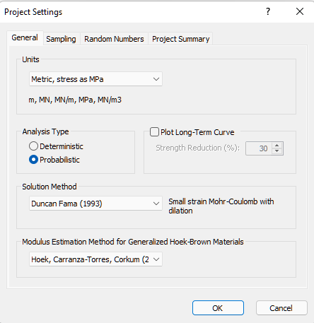
3. In the Project Summary tab change the Project Title to "Tutorial 3 Probabilistic Analysis."
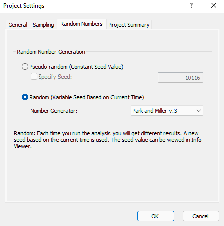
4. Ensure the Pseudo-Random number generation option is selected from the Random Numbers tab and click OK.

We will examine the Pseudo-Random number generation option and its purpose later on in the tutorial.

2.2 Tunnel and Rock Parameters

To open the Tunnel and Rock Parameters dialog:

1. Select: Analysis > Tunnel Parameters

Notice that the Tunnel and Rock Parameters dialog is presented in a grid format for a Probabilistic analysis. This simplifies the input of statistical parameters, and allows you to easily define random variables and keep track of which variables have been assigned statistical distributions.

2.2.1 RANDOM VARIABLES

To define a random variable, we first select a statistical distribution for the variable (e.g. Normal) in the Tunnel and Rock Parameters dialog. Then we enter the mean, standard deviation and relative minimum and maximum values, which define the statistical distribution for the variable.

It is important to note that the Minimum and Maximum values are specified as RELATIVE distances from the mean, rather than as absolute values. This simplifies the data input of these values.

For example: if the mean Friction Angle = 25 degrees, and the minimum = 20 and maximum = 30, then the relative minimum = 5 degrees and the relative maximum = 5 degrees.

For this example, we will define the following variables as random:

• In-Situ stress
• Young’s Modulus
• Compressive Strength
• Friction Angle

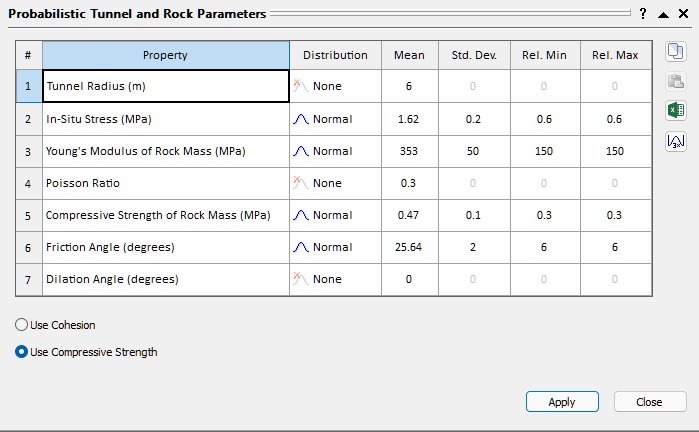
1. Enter the following data:

The Tunnel and Rock Parameters dialog should appear as follows.

2.2.2 AUTOMATIC MINIMUM AND MAXIMUM VALUES

You may have noticed that the relative minimum and maximum value we entered for each variable, was 3 times the standard deviation. For a Normal distribution, this ensures that a complete (non-truncated) distribution is defined (i.e. since 99.7% of all samples fall within 3 standard deviations of the mean, for a normally distributed random variable).

In the Tunnel and Rock Parameters dialog, the following shortcut can be used for this purpose (this is left as an optional exercise to experiment with, after completing this tutorial):

1. Enter the standard deviation for a random variable.
2. Select the button in the dialog, and the relative minimum and relative maximum for the variable will be automatically set to 3 times the standard deviation.

You can use this shortcut for multiple variables simultaneously – just use the mouse to first select all of the desired variables in the dialog, and then select the 3x button.

3. Now select Apply. This will save the parameters you have just entered, and run the RocSupport probabilistic analysis. The analysis should only take a few seconds or less (remember that we used the default Number of Samples = 10000 in the Project Settings dialog).
4. Close the Tunnel and Rock Parameters dialog, and we will view the analysis results.

3.0 Tunnel Section View

To select the Tunnel Section View:

1. Select: Analysis > Tunnel Section

The Tunnel Section View, for a Probabilistic analysis, appears the same as for a Deterministic analysis. However, in the analysis summary provided in the Project Info Textbox, note that:

• The results are the MEAN values from the statistical analysis. In general, these MEAN values will NOT NECESSARILY be the same as the Deterministic analysis results, based on the mean input data.
• A Probability of Failure, for the support, is listed, as well as the MEAN safety factor. The Probability of Failure represents the number of analyses, in which the Factor of Safety for the support was less than 1, divided by the total number of analyses (10000 in this case).

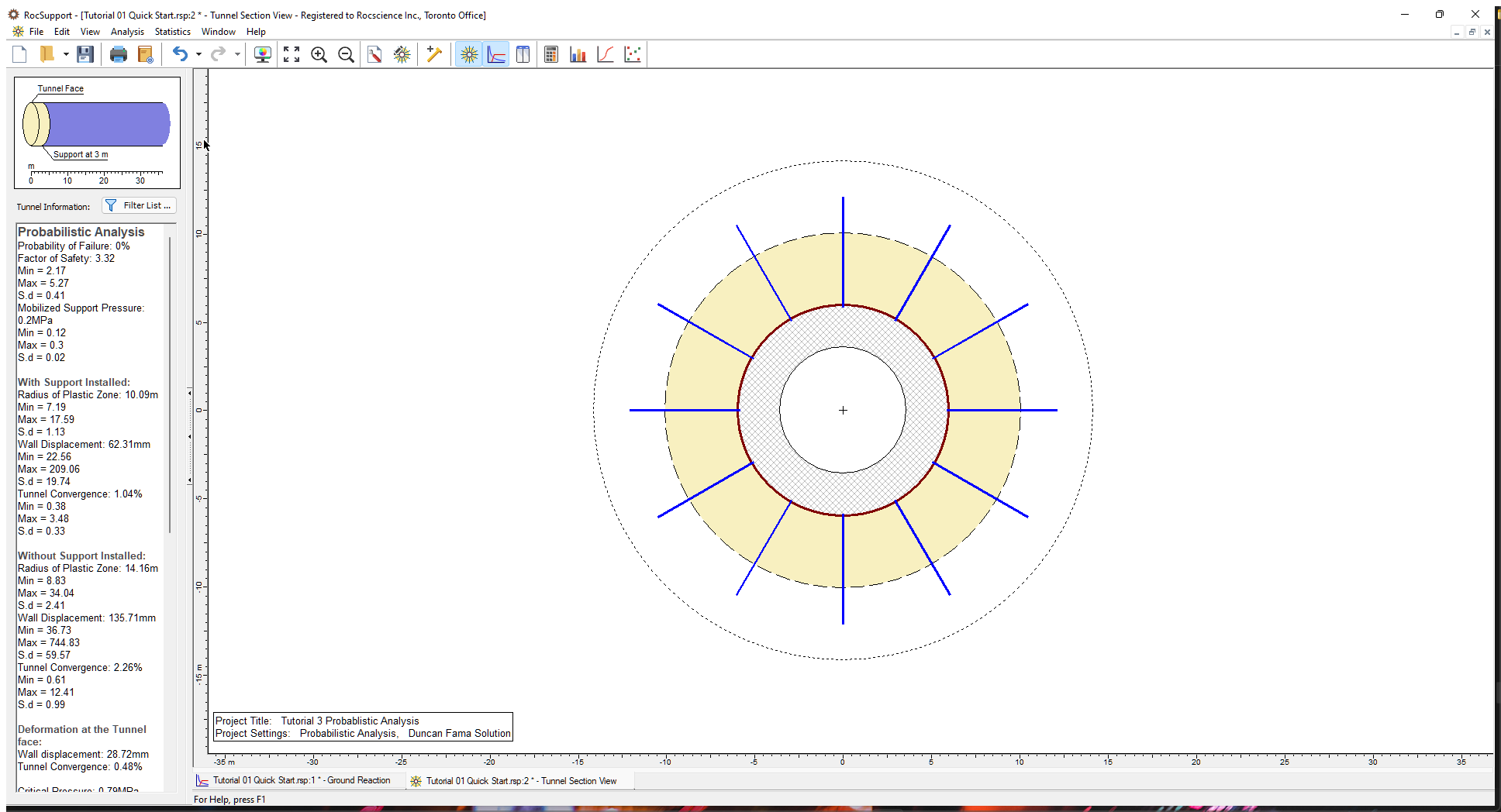
The Probability of Failure is currently zero (i.e. Factor of Safety is greater than 1 for all cases analyzed).

4.0 Statistics

After a probabilistic analysis, the user can plot the results in the form of Histograms, Cumulative Distributions, or Scatter Plots of input and output variables.

4.1 Histogram Plots

To create a Histogram plot:

1. Select: Statistics > Histogram Plot

(Alternatively, you can also activate the Histogram Plot dialog by pressing F7.)

Note that both input and output variables are listed in the Variable to Plot list.

• The output variables will always include Factor of Safety, Tunnel Convergence, Wall Displacement and Plastic Zone Radius.
• The input variables listed, will only be those for which you have entered a statistical distribution, in the Tunnel and Rock Parameters dialog. For our current example, this includes In-Situ Stress, Young’s Modulus, UCS of Rock Mass, and Friction Angle.

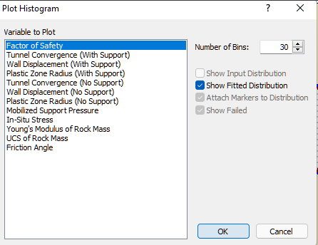
2. Let’s plot a histogram of Factor of Safety. Since this is the default selection in the Plot Histogram dialog, just select OK to generate the plot.

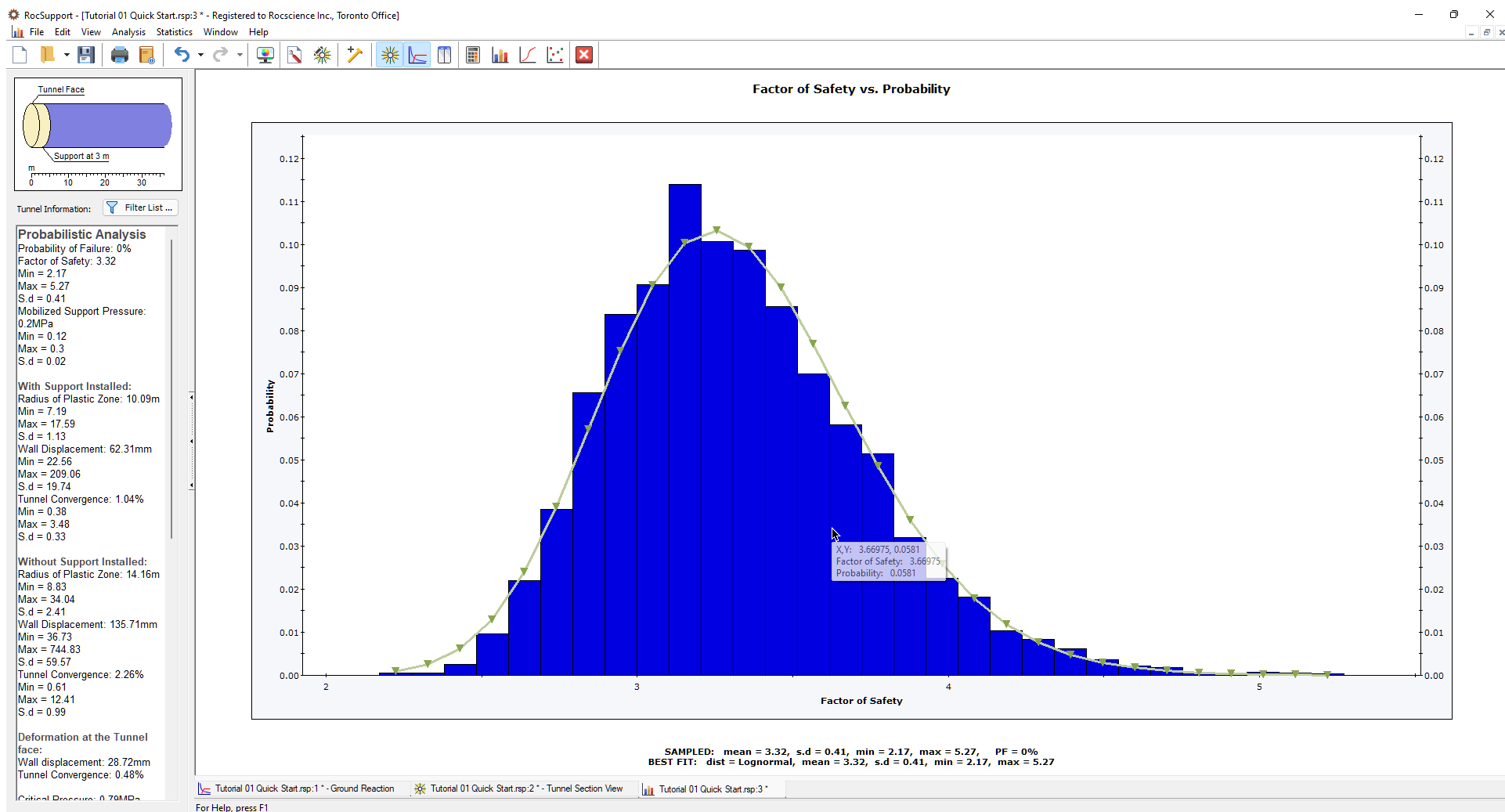
As you can see in this plot, there were no analyses with a Factor of Safety less than 1. The Probability of Failure is therefore zero.

For calculated output variables such as Factor of Safety, a FITTED distribution can be displayed on a histogram, as shown in the above figure. The fitted distribution can be toggled on or off in the right-click menu, the Statistics menu or in the Plot Histogram dialog (select the Show Fitted Distribution option). The Fitted Distribution represents a best-fit distribution for the output variable, and is automatically determined by RocSupport. Note that the Fitted Distribution can be any one of the statistical distributions used in RocSupport (i.e. normal, uniform, triangular, beta, exponential, lognormal or gamma).

Now let’s generate a histogram of one of our input variables, for example, In-Situ Stress.

1. Select: Statistics > Histogram Plot
2. In the Plot Histogram dialog, select In-Situ Stress from the Variable to Plot list.
3. Select OK.

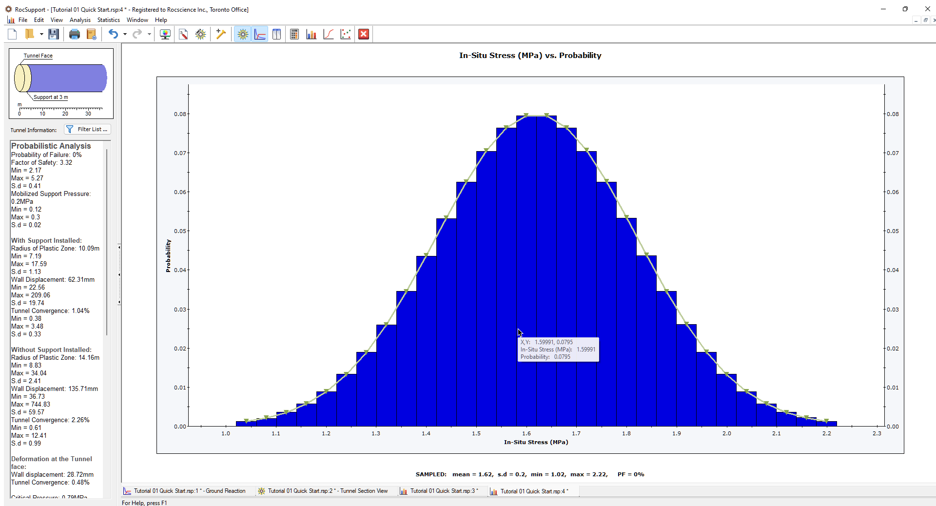
For input variables, the Input Distribution can be displayed on the Histogram plot, as shown in the above figure for In-Situ Stress. Also a statistical summary of the simulated values, and the parameters of the Input Distribution are provided at the bottom of the plot.

• The Input Distribution is the distribution defined by the input data you have entered in the Tunnel and Rock Parameters dialog.
• The Sampled data statistics are derived from the raw data generated by the statistical sampling (Latin HyperCube method in this case) of the Input Distribution you have defined.

This explains why the SAMPLED and INPUT statistical parameters listed at the bottom of an input variable histogram, will in general differ slightly, especially if the Number of Samples is small.

4.2 Cumulative Plots

A cumulative distribution is, mathematically speaking, the integral of the normalized probability density function. Practically speaking, a point on a cumulative distribution gives the probability that a random variable will be LESS THAN OR EQUAL TO a specified value.

To generate a Cumulative distribution:

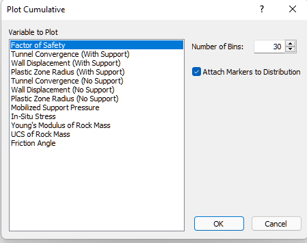
1. Select: Statistics > Cumulative Plot

Note that the list of Variables to Plot, is exactly the same in both the Plot Histogram and Plot Cumulative dialogs.

2. Let’s plot the Factor of Safety cumulative distribution. Since this is the default selection in the Plot Cumulative dialog, just select OK to generate the plot.

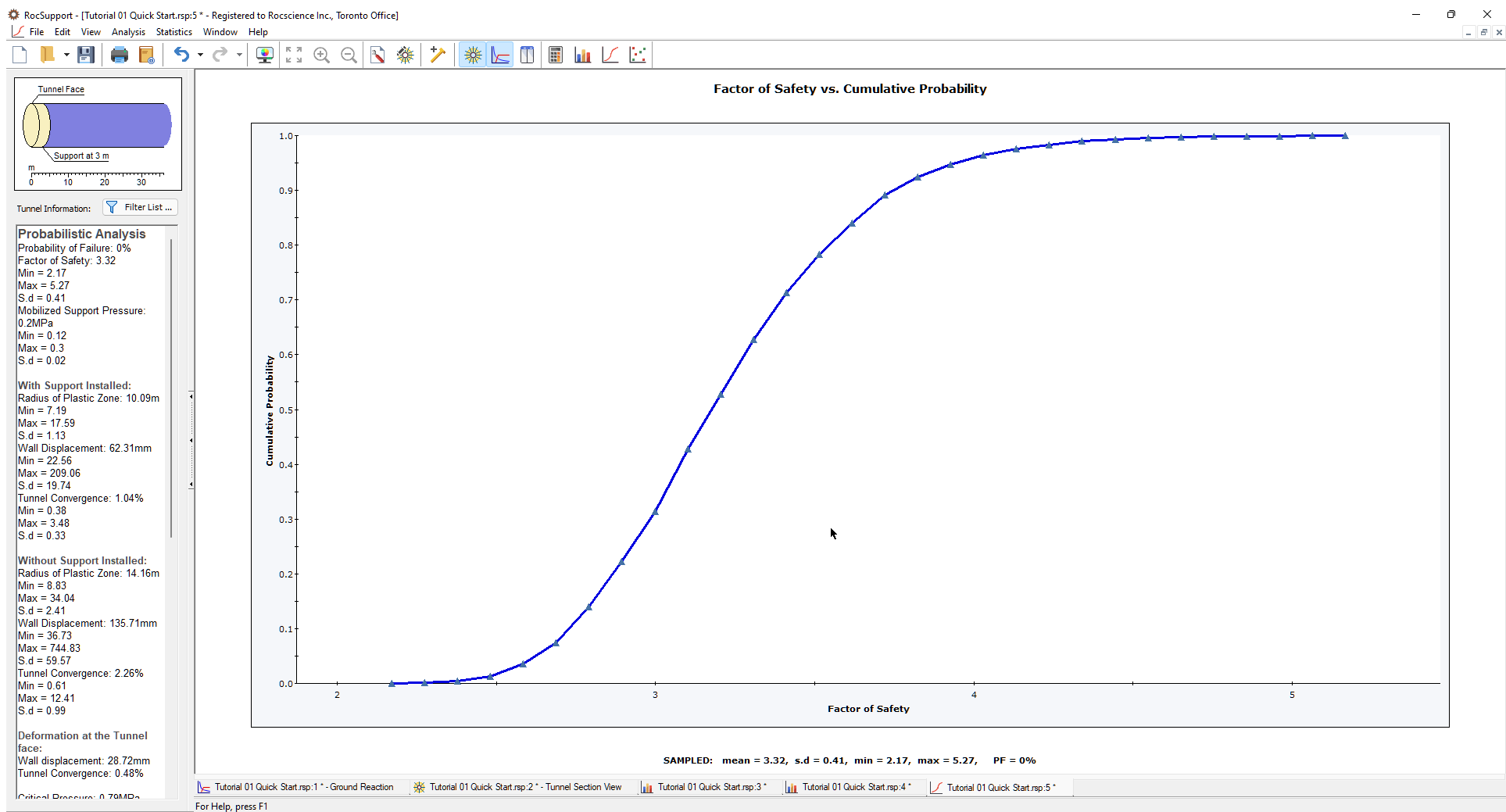
It is worthwhile noting that for the cumulative distribution of Factor of Safety, the cumulative probability at Factor of Safety = 1, is equal to the Probability of Failure. In this example, the Factor of Safety is greater than 1 for all cases, therefore the Probability of Failure = 0.

4.3 Scatter Plots

Scatter plots can also be generated after a probabilistic analysis. Scatter plots allow you to plot any two random variables against each other, to view the correlation (or lack of correlation) between the two variables.

1. Select: Statistics > Scatter Plot
2. In the Scatter plot dialog, select Factor of Safety versus In-Situ Stress.

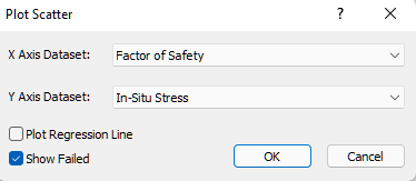
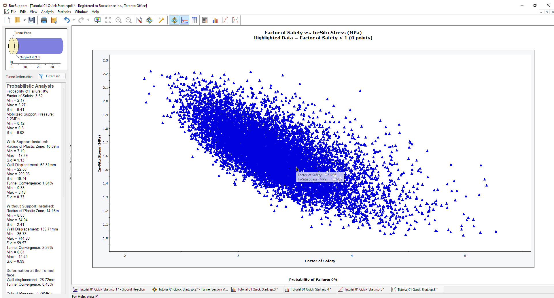
It can be seen that there is a general correlation between the input variable In-Situ Stress, and the Factor of Safety for the support. The best fit linear regression line can be displayed using the right-click menu shortcut, if desired.

5.0 Computing the Analysis using True Random Sampling

For this tutorial, we selected the Pseudo-Random Sampling option from the Random Numbers tab in the Project Settings dialog. Therefore, when the Apply button is clicked in the Tunnel Parameters or Support Parameters dialogs, RocSupport uses PSEUDO-RANDOM numbers to generate the statistical sampling of the input variable distributions. Pseudo-random sampling generates the SAME RESULTS each time the analysis is run. This allows the user to obtain reproducible results for a Probabilistic analysis.

To run a Probabilistic analysis using TRUE RANDOM sampling, then you must select the Random sampling check box in the Random Numbers tab of the Project Settings dialog.

With Random sampling, different random numbers are used to generate each sampling of the input variable distributions. This means that EACH TIME COMPUTE or APPLY is selected, different results will be generated.

We will re-run our example using true random sampling and observe the results.

1. Select: Analysis > Project Settings
2. In the Random Numbers tab, select the Random check box and click OK. The analysis is immediately recomputed, and results different from the previous ones are displayed.
   
3. To observe the effect on the Scatter Plot, select the Compute button several times (or select Statistic > Compute from the menu).

The graph is updated after each Compute, to reflect the latest results.

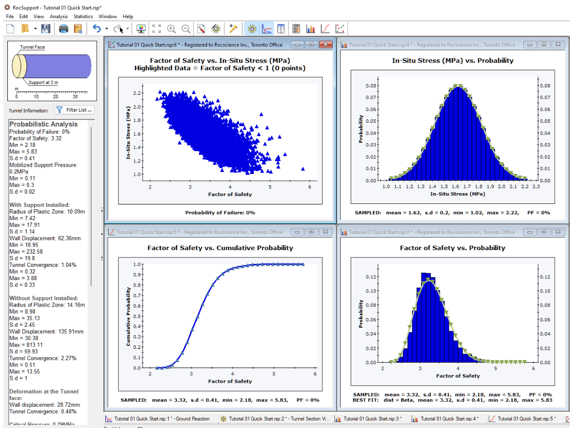
To further illustrate the results of using Compute with true random sampling, let’s tile the views.

4. Select: Window > Tile Vertically
   
5. If you have followed the steps in this tutorial, and did not have any other RocSupport files open, you should have six views open. Close two of the views (for example, the Ground Reaction View and the Tunnel Section View) so that only the statistical plot views are open.
6. Select the Tile option again, and your screen should look similar to the figure below.

6.0 Additional Exercise

Although we demonstrated the Probabilistic analysis features of RocSupport in this tutorial, the Probability of Failure was zero!

As a final exercise, we will create an example with a Probability of Failure greater than zero, in order to demonstrate some additional graphing features of RocSupport.

1. In the Support Parameters dialog:
   • Remove the Shotcrete support completely, by clearing the Shotcrete check box
   • Change the Rockbolt type to 19 mm rockbolt. Select Apply and Close.
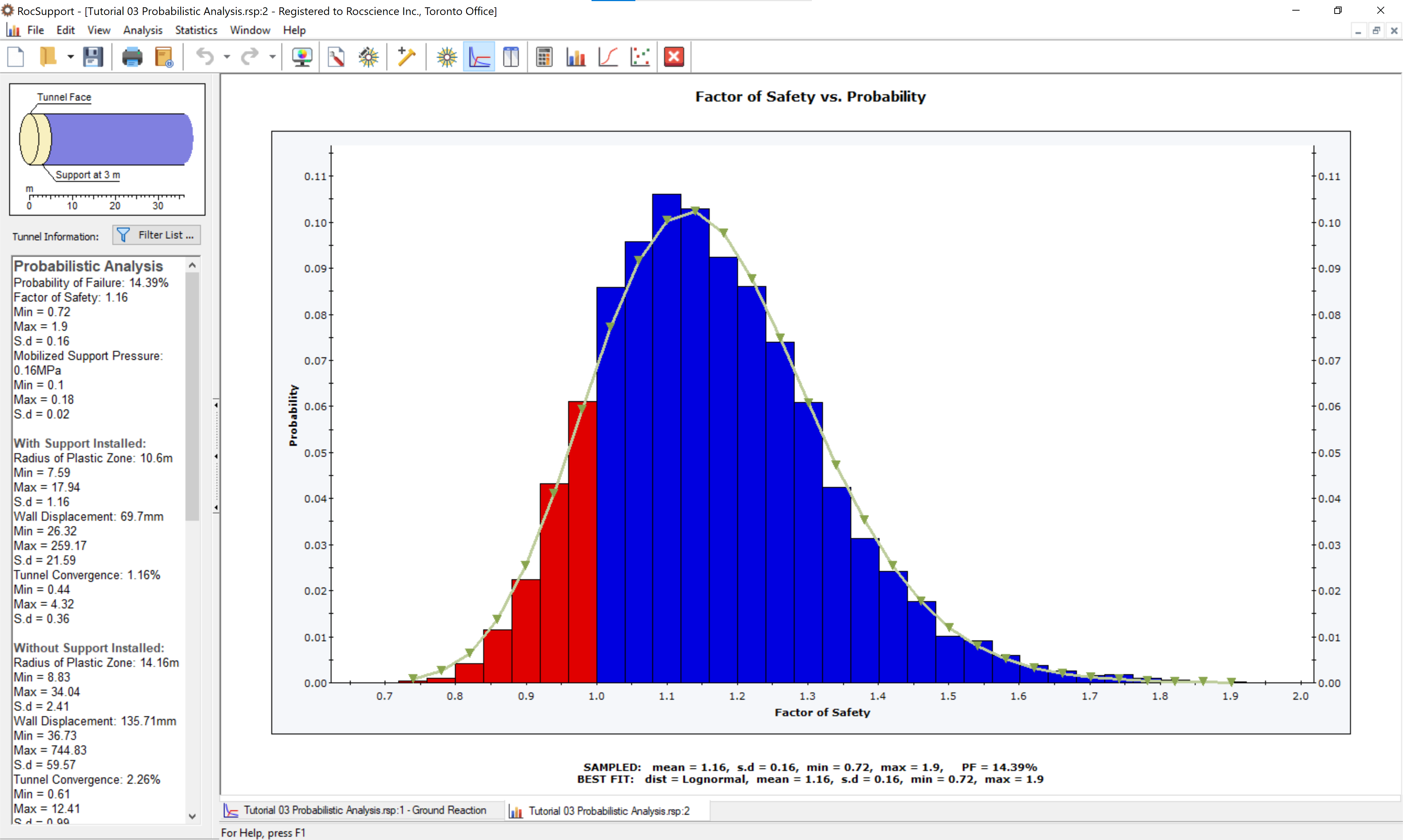
2. View the Safety Factor Histogram. Notice that all bars with a Factor of Safety less than 1, are now highlighted in RED. Note that the Probability of Failure (PF) listed at the bottom of the histogram, is greater than zero, indicating a finite probability of failure.
   
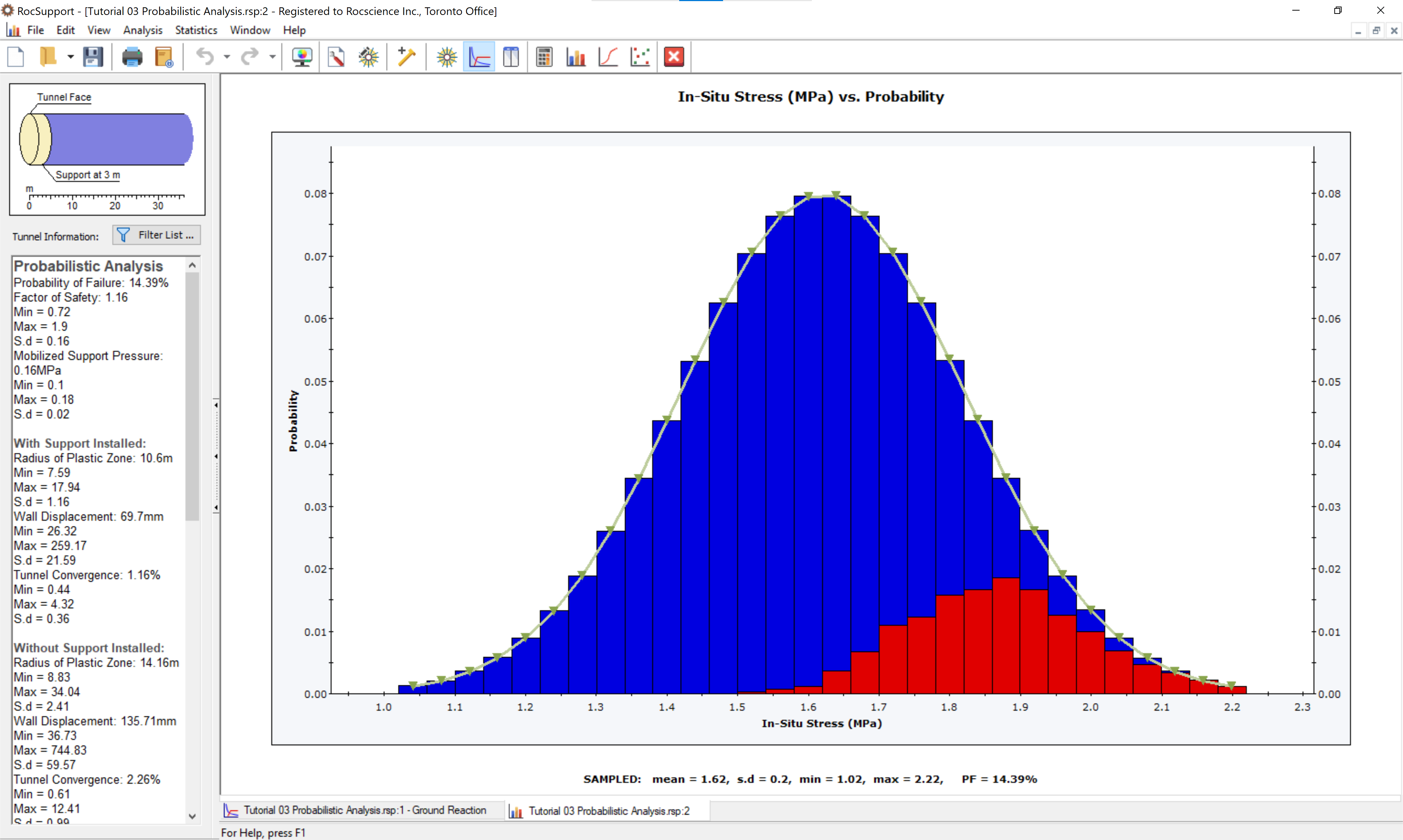
3. View the In-Situ Stress Histogram. The percentage of each bar of the histogram, corresponding to analyses with Factor of Safety less than 1, is now highlighted in RED.
   NOTE: the display of failed data on histograms can be toggled on or off by selecting the Show Failed Bars option from the Statistics menu or the right-click menu.
4. Re-select Compute several times. Notice that all views are updated to reflect the latest results.
5. Repeat steps 3 to 5 for other input or output variables. Notice the distribution of failed analyses, with respect to the overall distribution of the variable.

The Show Failed Bars option allows you to examine the relationship of any given input or output variable, to the failure of the support system.

That concludes the probabilistic analysis tutorial.