21 - Pile Resistance Using RSPile

1.0 Introduction

In this tutorial, we will demonstrate how to improve the stability of a slope using pile supports from RSPile.

We will analyze the following two scenarios in Slide2:

• Scenario 1 will analyze the stability of an unsupported slope
• Scenario 2 will analyze the stability of the same slope, which has been reinforced with piles
• We will then verify the pile resistance using RSPile

The finished product of this tutorial can be found in Tutorial 21 Pile Resistance using RSPile.slmd data file. All tutorial files installed with Slide2 can be accessed by selecting File > Recent Folders > Tutorials Folder from the Slide2 main menu.

2.0 Geometry Model

1. Select File > Recent Folders > Tutorials Folder from the Slide2 main menu and open Tutorial 21 Pile Resistance using RSPile – starting file.slmd.

In the model, the two scenarios discussed above have already been created. The slope material properties are also defined in the material properties dialog. (See Properties > Define Materials)

We will now run the first scenario (No support).

2. In the Document Viewer, click on the first scenario and select Analysis > Compute to run the analysis. Select Analysis > Interpret to view results when computations are done.

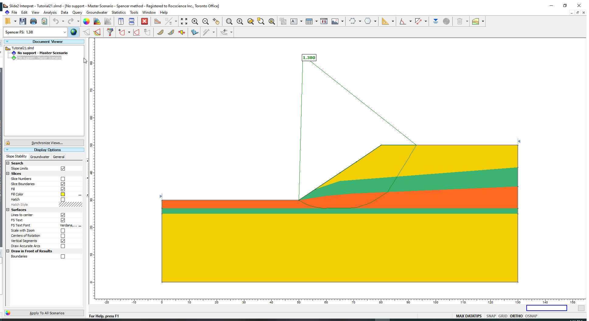
From the analysis, the safety factor of the critical slip surface is approximately 1.4, which is lower than our design target of 1.5. The slope safety factor can be improved using Pile support.

3.0 RSPile Support

First, we will define Pile support for the slope in Slide2. Begin by returning to the Modeller.

1. Select Properties > Define Support to open the Define Support Properties dialog.
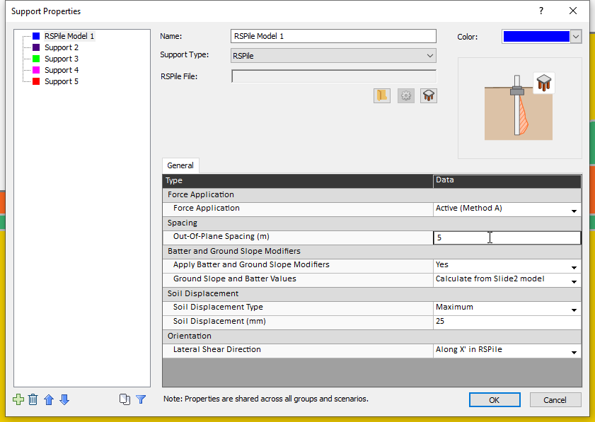
2. In the dialog, select Support 1 and define the following properties.
   1. Name: RSPile Model 1
   2. Support Type: RSPile
3. Under the General tab:
   1. Force Application: Active (Method A)
   2. Out-of-Plane Spacing (m): 5
   3. Apply Batter and Ground Slope Modifiers: Yes
   4. Ground Slope and Batter Values: Calculate from Slide2 model
   5. Soil Displacement Type: Maximum (The Maximum mode assumes that a maximum allowable soil displacement of 25 mm in the direction tangent to the tested slip surface is used to compute the axial and lateral resistance against sliding. Meanwhile, the Ultimate mode increases the applied soil displacement in the axial and lateral direction until a maximum resistance is reached.)
   6. Soil Displacement: 25 mm
   7. Use Angle Divisions: Enabled
   8. Lateral Shear Direction: Along X’ in RSPile (soil displacement analysis will be carried out along the X’ direction of the RSPile)

For piles that are not radially symmetric, you can change this setting to apply the lateral displacement along either of the major axes (X’ or Y’) of the pile.

For more information about these settings, see the RSPile help page.

We will now design the Pile support using RSPile.

To run RSPile:

1. Click on the RSPile icon immediately below the input field labelled ‘RSPile File’. (Alternatively, you can run the RSPile model program by double-clicking on the RSPile icon in your installation folder.) The RSPile program interface will open as shown below.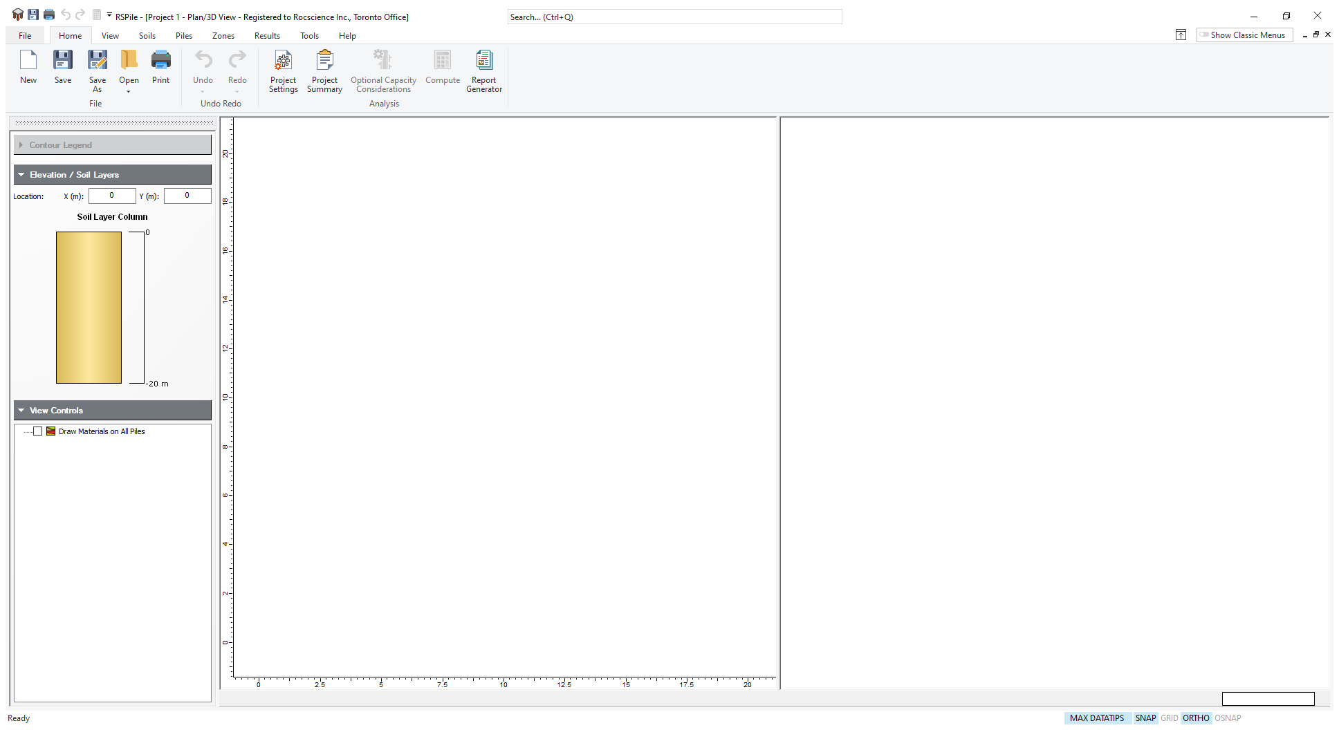

   

2. In RSPile, select Home > Project Settings to open the Project Settings dialog.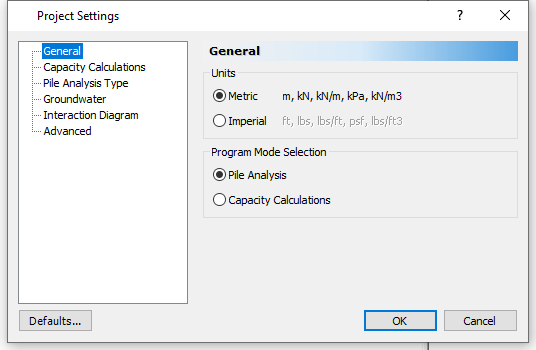

   

3. In the General tab ensure the unit system is set to SI (Metric).
4. Select the Pile Analysis Type tab. Ensure the Pile Analysis Type is set to the Individual Pile Analysis mode, and from the dropdown select Axially/Laterally Loaded. This choice means that the slope piles will be subjected to axial and lateral loads.
5. Uncheck the box for Include P-Delta Effect.
6. Click OK to save the settings and close the dialog.

Next, we will define the properties of the materials in the slope.

4.0 Soil (Material) Properties

Each soil property will be divided into Axial and Lateral. Some soil properties are common between laterally or axially loaded piles, for example, names, unit weights, and colours. Other properties that may be common within one base type, such as friction angle for any sand, are not copied between modes because the material models are different and usually contain unique property values depending on the problem.

We will enter properties under the Axial and Lateral tabs.

1. Select Soils > Define Soil Properties to open the Soil Properties dialog.

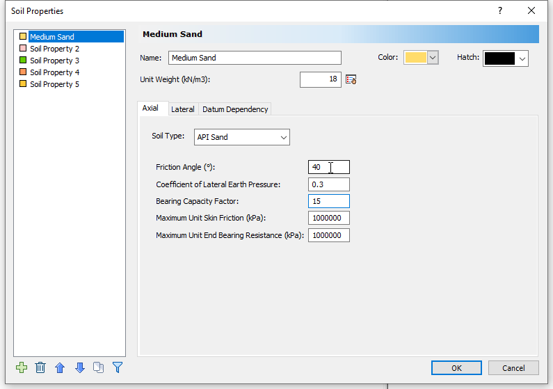
2. For Soil Property 1 enter the following properties.

   1. Name: Medium Sand
   2. Unit Weight (kN/m3): 18
   You do not need to define the layer thicknesses because these values will be initialized according to the soil profile of the installed pile support in Slide2. As such, we can use one RSPile model file to define the soil and pile properties for multiple piles of various embedment lengths and soil layer configurations.

3. Click on the Axial tab and enter the following parameters in the respective fields:

   1. Friction Angle: 40
   2. Bearing Capacity Factor: 15
   3. Maximum Unit Skin Friction: 1000000
   4. Maximum Unit End Bearing Resistance: 1000000

   

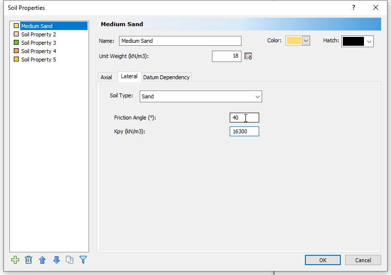
4. Next, click on the Lateral tab and enter the following parameters in the respective fields:

   1. Soil Type: Sand
   2. Friction Angle (degrees): 40
   3. Kpy (kN/m3): 16300

   

5. Now click on Soil Property 2, and enter the name, unit weight and axial properties from the table below. We will use an example of a typical non-linear t-z curve based on empirical data values for this material.

   Name	Dense Sand
   Unit Weight	20
   Axial Tab
   Soil Type	User Defined
   Ultimate Skin Friction (kPa)	43
   Ultimate Unit End Bearing Resistance (kPa)	0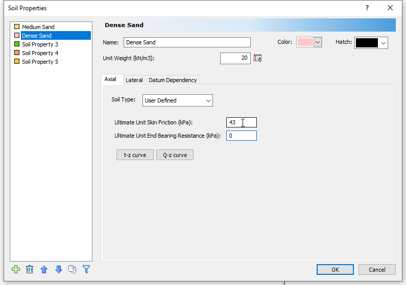

   

6. Click t-z curve and enter the Displacement (mm) and Stress to Max Ratio:

   Displacement (mm)	Stress to Max Ratio
   0	0
   0.28	0.4
   0.476	0.6
   0.561	0.675
   0.695	0.76
   0.854	0.83
   1.1	0.9
   1.4	0.935
   1.74	0.965
   1.95	0.972
   3.05	1

7. Click OK to close the t-z curve table and return to the Soil Properties dialog. You do not have to define the Q-z curve for this tutorial since it is assumed that this soil layer has no end bearing strength.

8. Under the Lateral tab set the Soil Type as User Defined and click on the p-y curve button. This will open the ‘p-y’ curve table. (A p-y curve relates soil reaction to pile deflections at points along the length of a pile)

   

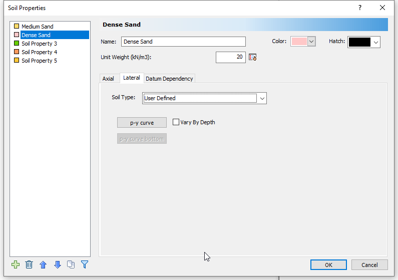
9. Enter the following values in the table:

   Displacement (mm)	Soil Resistance (kN/m)
   0	0
   1	300
   20	1800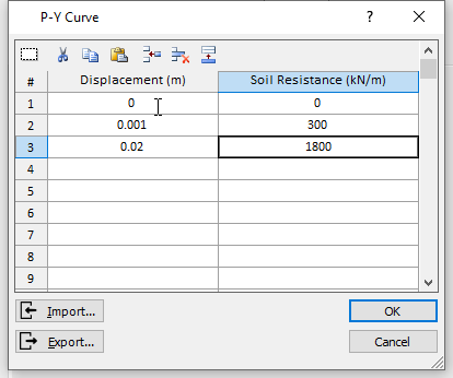

   

10. Click OK to close the dialog.

11. Now let us define the parameters for the last soil material, Soft Clay.

    1. Name = Soft Clay
    2. Unit Weight = 17
    3. Axial tab
       1. Soil Type = API Clay
       2. Undrained Shear Strength = 82
       3. Remolded Shear Strength = 82
       4. Maximum Unit Skin Friction = 1000000
       5. Maximum Unit End Bearing Resistance = 1000000

    

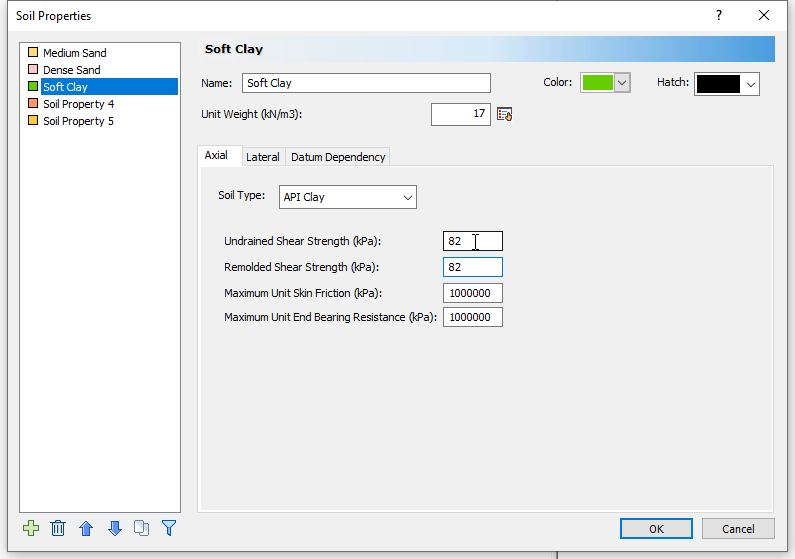
    1. Lateral tab

       1. Soil Type = Soft Clay Soil
       2. Strain Factor = 0.007
       3. Undrained Shear Strength = 82

       

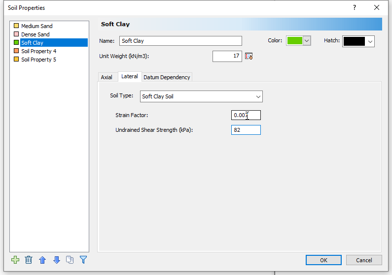
12. Click OK to save settings and exit the dialog.

We have now defined all the soil materials. The next step is to define a borehole with these soil layers.

5.0 Edit All Boreholes

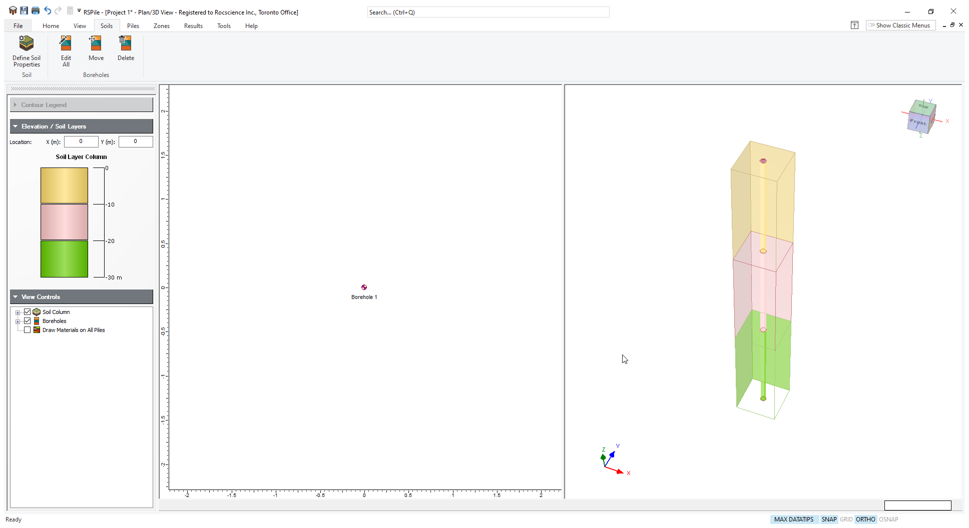
1. Select Soils > Edit All (Boreholes) to open the Edit Borehole dialog. By default, only the first soil type (Medium Sand) we created is shown. We will add the other two layers.
2. Click Insert Layer Below twice. The program will automatically add the two materials.

3. Enter the layer thicknesses shown in the table below.

   Name	Thickness (m)
   Medium Sand	10
   Dense Sand	10
   Soft Clay	10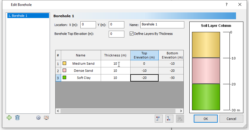

   

4. Click OK to close the borehole dialog.

A borehole profile, representing the stratigraphy we just defined, will now appear in the Plan and 3D views of the software as shown below.

Next, we will define the structural properties of the pile in the Pile Section Properties dialog.

6.0 Pile Section Properties

1. Select Piles > Pile Sections to open the Define Pile Section Properties dialog.

2. Select Pile Section 1 and enter the following properties:

   Name	Steel Pipe
   Section Type	Elastic
   Young’s Modulus (MPa)	2e5
   Cross Section	Pipe
   Pipe Outside Diameter	0.61
   Pipe Wall Thickness	0.02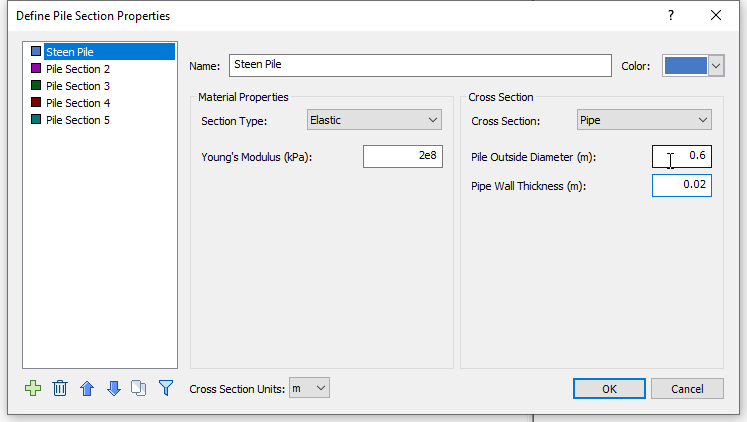

   

3. Click OK to close the dialog.

   We will install the pile in the soil profile.

4. Select Piles > Single to bring up the Add Pile dialog.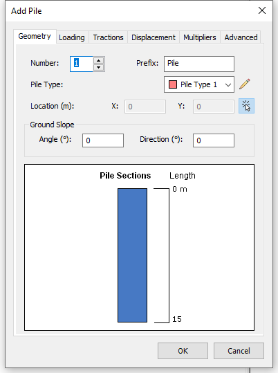

   

5. Under the Geometry tab, click on the Edit Pile Type button (pencil icon). In the resulting Edit Pile Types of dialog, Pile Type 1 is assigned the Steel Pipe section property we defined earlier.
6. Enter a Steel Pipe length of 21m.
   
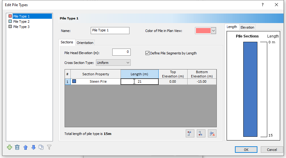
7. Click OK to close the Edit Pile Type and Add Pile dialogs. RSPile will prompt you to enter a location (in plan view) for the head of the pile.
8. If prompted, enter (0,0) in the Prompt line to place the pile and press Enter. (When the pile design is imported into Slide2, the piles will be placed at the locations specified in Slide2.)

Now we will save our RSPile file and import it into the Slide2 model.

9. Select File > Save As and save file as Tutorial 21 Pile Resistance using RSPile.rspile2 on your computer.

7.0 Importing RSPile Model into Slide2

Return to your Slide2 Tutorial 21 file.

1. In the Support Properties dialog, click the folder icon below the RSPile File field. (Select Properties > Define Support to open it if you closed it.)

2. Open Tutorial 21 Pile Resistance using RSPile.rspile2.

   The Match Slide2 and RSPile Materials dialog appears as shown below.

3. In the dialog, tick the Show only used Slide2 materials checkbox, and ensure that the materials in Slide2 are matched to their RSPile counterparts as shown below.

   

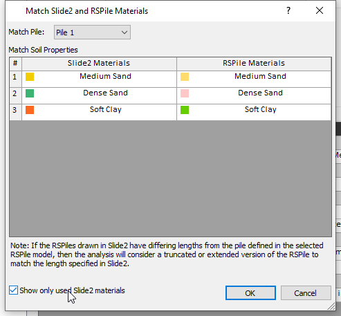   Written warnings may be generated during the import process and shown at the bottom of the dialog. As discussed in an earlier note, the pile lengths in Slide2 will be 21m and 25m even though the RSPile pile length was 21m.
4. Click OK to close the dialog.

Now we are ready to compute the analysis.

8.0 Computation and Interpretation of Results

1. Click on the Pile support scenario and note the location of the piles.
2. Run the analysis (Analysis > Compute ) and view results (Analysis > Interpret ) when Slide2 computations are done.

The Slide2 engine appears, which in turn calls up the RSPile compute engine. After Pile Analysis is completed, the RSPile engine automatically passes the pile resistance forces to Slide2 for slope stability calculations.

3. Select Data > Show Support Force Diagram to turn on the Support Force diagram.

You should see the following figure for the Spencer FS analysis.

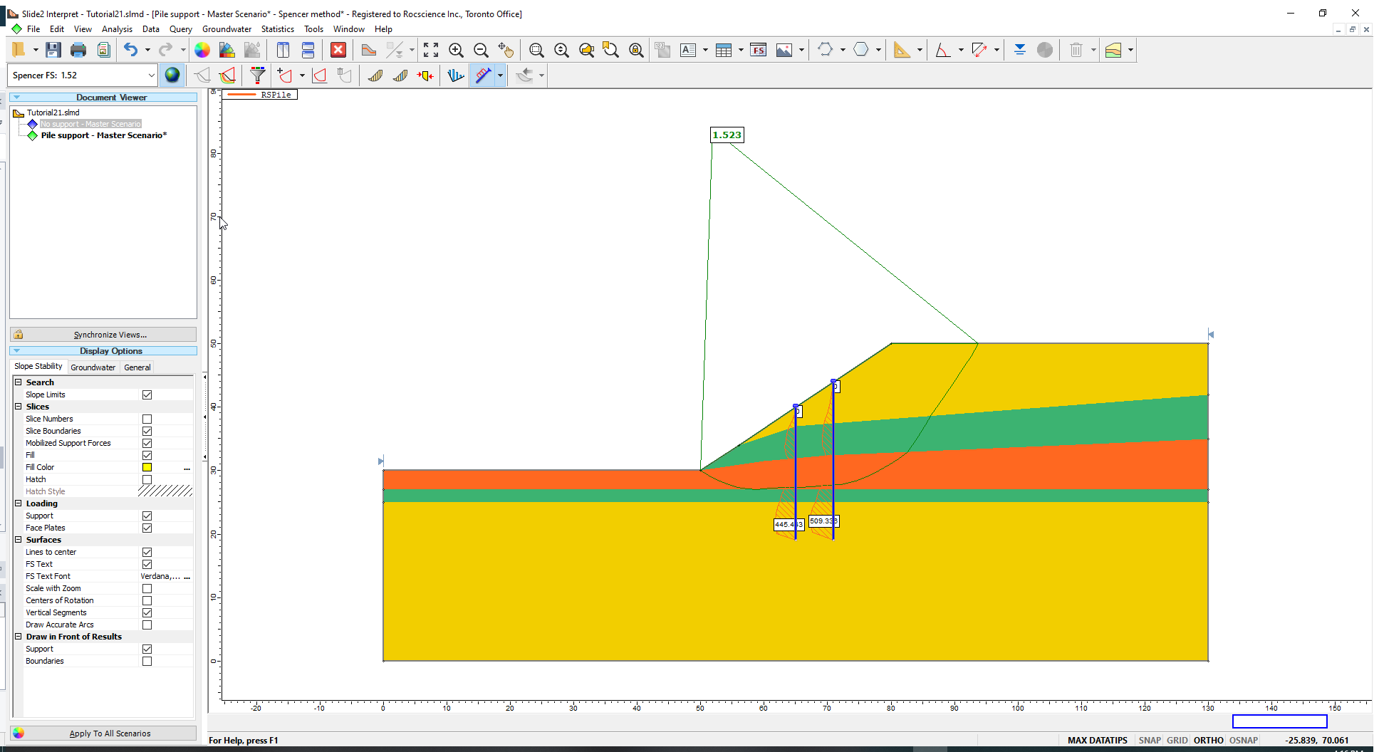
The safety factor of the critical surface has improved with the addition of Pile Supports.

4. Select Query > Show Slices to view the pile resistance forces acting on the critical slip surface.

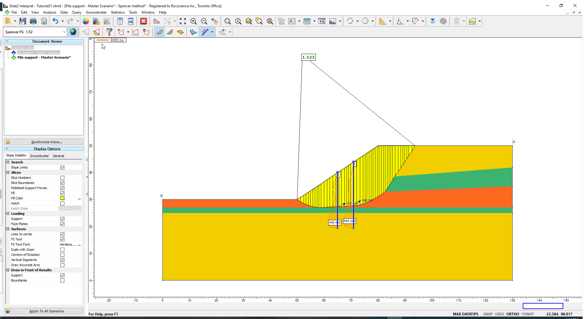
The pile resistance is indicated by the blue arrow with its origin located at the intersection of the pile and slip surface. Notice that the direction of pile resistance is always opposite to the direction of sliding although it may not always be tangent to the slip surface. Each slip surface analyzed will have a different pile resistance depending on the depth and angle of intersection.

Note that because the pile out-of-plane spacing is 5 m, the actual force for each pile is 5 times higher.

This part of the tutorial is now complete.

9.0 Additional Exercise: Verifying Pile Resistance using RSPile

You can verify the pile resistance results from Slide2 by using the same pile length and soil layer configuration for the RSPile model. For this tutorial, we will be verifying the pile resistance of the downslope, shorter pile. We will check whether the Slide2 pile resistance profile matches that from RSPile for the left pile.

We will develop an RSPile model using the soil layering from Slide2, and then compare the model’s results to the Slide2 pile resistance.

Note that this analysis will be completely run in RSPile.

1. Return to the RSPile Model program and open the Tutorial 21 Pile Resistance using RSPile.rspile2 file if it is not already open.

2. Go to Soils > Edit All Boreholes dialog and change the soil layer thicknesses to the following (to exactly match the stratigraphy at the location of the left pile in Slide2):

   Name	Thickness
   Medium Sand	3
   Dense Sand	5
   Soft Clay	5
   Dense Sand	2
   Medium Sand	6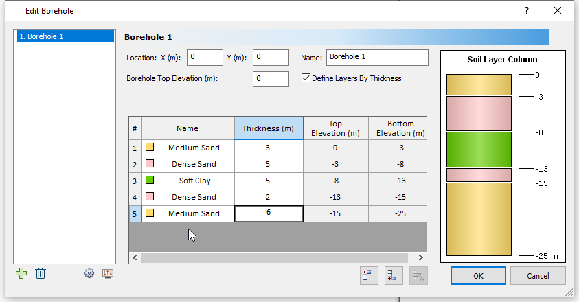

   

3. Click OK to close the dialog.

9.1 PILE RESISTANCE

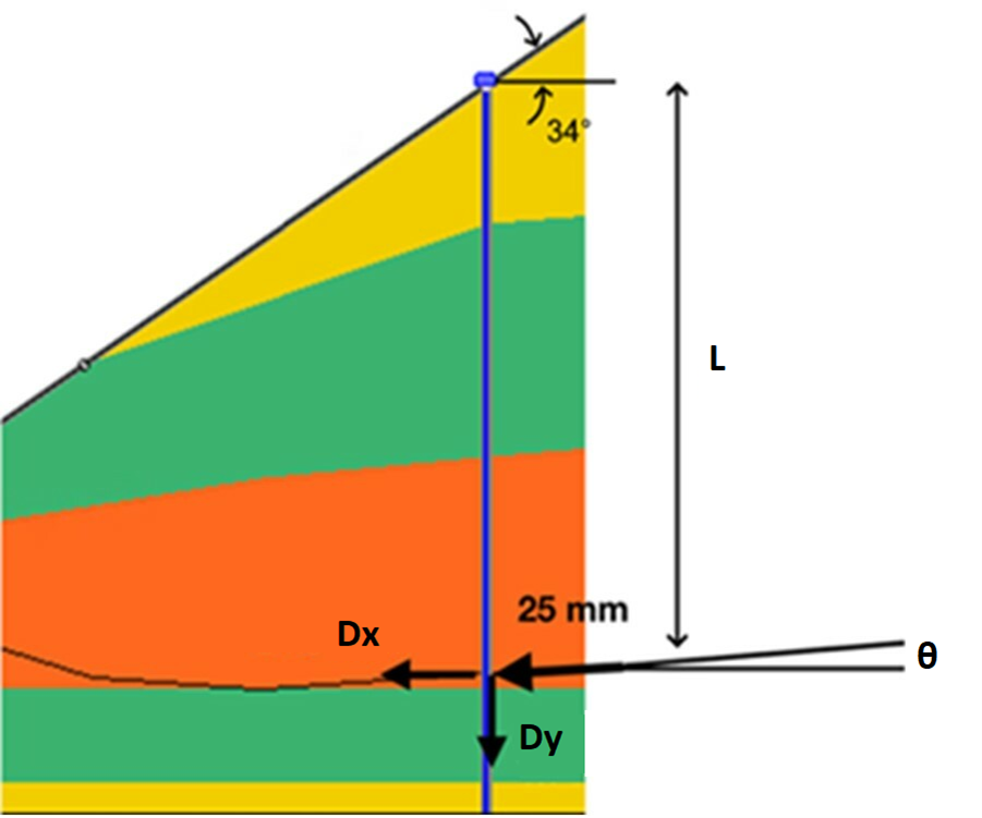
1. In Slide2, take note of the resistance force for the left pile (which is shown when Show Slices is enabled) – call this R’. This will be split into lateral and axial components Fx’ and Fz’ respectively.
2. Use the Tools > Dimension Angle option to measure the angle of the slip surface as it intersects the left pile – call this θ.
3. Measure the distance from the top of the pile to the point of intersection with the slip surface – call this L.

4. The maximum soil displacement input into Slide2 to calculate pile resistance is 25 mm. Resolve this into vertical and horizontal component using θ (i.e., Dy and Dx in the diagram).

   Most of this information can also be obtained by using the Query > Query Slice Data feature and selecting the slice containing the pile.

5. The variables are shown schematically below:
   

   We will now enter the above information into RSPile.

6. Right-click on the pile in the Plan view and select Edit Pile.
7. Go to the Displacement tab in the Edit Pile dialog:
8. Ensure you have selected the Soil Displacement radio button
9. Enter the global displacements in the X and Z axes:
   Using the angle of the slice base measured in Slide2, resolve the maximum soil displacement to X and Z components. For example: 
   1. |d_x| = |25mm * cos(θ)|
   2. |d_z| = |25mm * sin(θ)|
      Note: Since the failure is occurring from right-to-left in Slide2 and the slice angle is positive, enter negative d_x and d_z values to simulate soil displacement downward and to the left as shown:
10. Input the Sliding Depth as the L measured from Slide2
11. Click OK to return to the Edit Pile dialog, and then switch back to the Geometry tab.
12. Change the Ground Slope angle to +34° and direction (bearing in the horizontal plane) to 90°. The direction of the ground slope is measured clockwise from the Y-axis (we can think of it as the north) in RSPile, and a positive Ground Slope angle dips downwards. Click OK
13. Recalculate by selecting Results > Compute
14. Right-click on the pile and select Graph Pile
15. Change the graph and table data so that you can see both Beam Shear Force X’ and Beam Axial Force. This is done as follows for the graph and table, respectively:
    1. Select Chart > Edit Charts Click on the second Chart Output and select Beam Shear Force X’ from the dropdown. Click on the third Chart Output and select Beam Axial Force. Click OK.
    2. Select Chart > Edit Table Columns Click Match to Charts select the same results data as the charts, and then click OK.

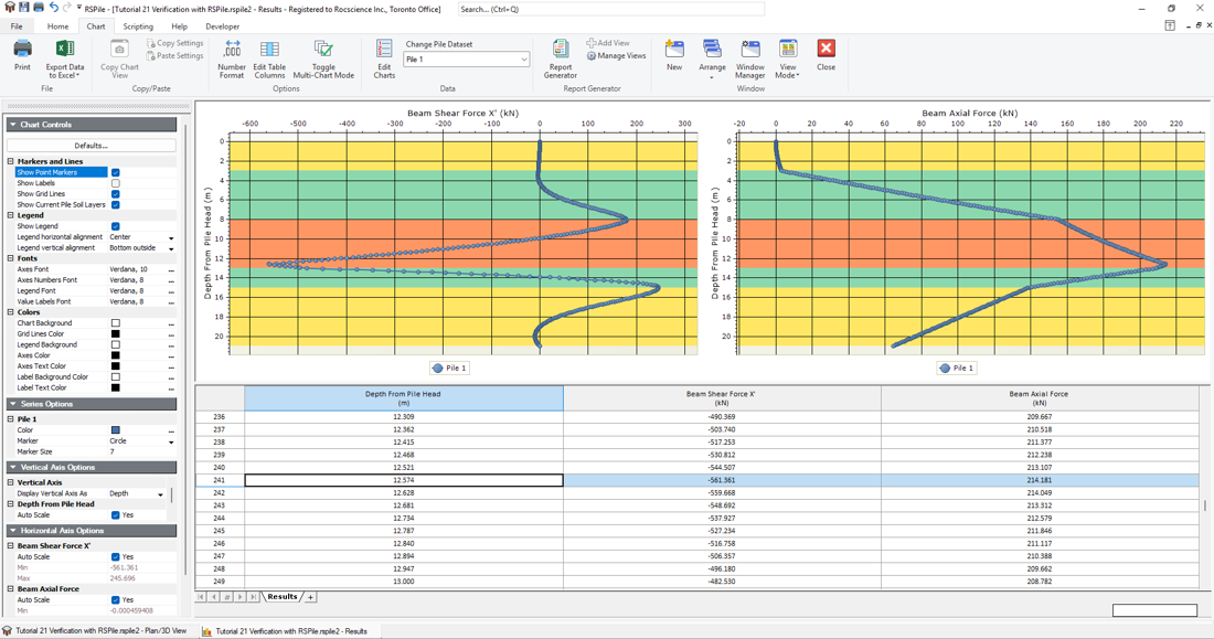
For example, at a depth of approximately 12.574m, the lateral and axial (Fx’ and Fz’) forces are -561.361kN and 214.181kN respectively.  Since the out-of-plane pile spacing was set as 5m in Slide2, we will divide the resultant by 5 to get the force on the individual pile.

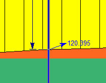
The slip surface intersected the pile at L m in Slide2 so we will look at the two depths, D1 and D2, such that D1<L<D2, recorded in the RSPile output and interpolate.

At a depth of D1, take down the shear force, Fx’1, and axial force, Fz’1. Calculate the resultant force, R1. At a depth of D2, do the same to get R2. Interpolate these to get the resultant, R at a depth of L.

Now go back to the R’ we obtained from Slide2. Recall that, due to the 5 m spacing, the program’s pile force should be multiplied by 5, yielding a magnitude of R_Slide2. Compare this force to the R obtained from RSPile. They should be very close.

Discrepancies are commonly due to the linear interpolation of the resistance at two locations, decimal precision, measurement, and/or pile segments used in RSPile’s FEA analysis. In Slide2, the resistance functions are constructed for the number of sliding depths as set in RSPile and the soil displacement is varied at each sliding depth to account for the unknown slip surface angle of intersection. First, linear interpolation is done to compute the resistance function for the exact component of soil displacement produced by the slip surface based on the closest tested soil displacements. Second, linear interpolation is done to compute the resistance for the exact sliding depth since the tested sliding depths are unlikely to align exactly with the actual slip surface intersection with the pile. With the angle division approach, the angle of the displacement is varied at each sliding depth rather than the magnitude of the displacement. This better accounts for any angle of slip surface intersecting the pile.

RSPile provides more control over the exact soil displacements and sliding depth since we are verifying a slip surface under analysis. However, repeating this resistance computation for every slip surface in Slide2 is rather tedious, necessitating an automated process. Even with a relatively low Number of Intervals, the resultant pile resistance computed in RSPile will be very close to that from Slide2 (within typically accepted tolerances).

9.2 ADDITIONAL EXERCISE - BATTERED PILE RESISTANCE

Similar to the vertical pile, we can verify the force for a battered pile. For the purposes of this example, we will only consider the left pile. 

1. Duplicate the existing group by right-clicking the scenario and selecting Duplicate Group.
2. Right-click the left pile, select Modify, and then change the angle to 290 degrees. 

3. Delete the right pile and click Compute as before, taking note of the same parameters as the previous example

   

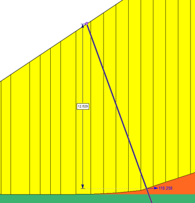
4. In either the existing or a new duplicated RSPile file, set the layers to the new vertical depths as shown:

   #	Name	Thickness (m)
   1	Medium Sand	2.918
   2	Dense Sand	4.835
   3	Soft Clay	5.246
   4	Dense Sand	2.009
   5	Medium Sand	4.724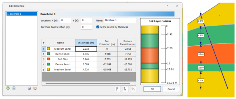

   

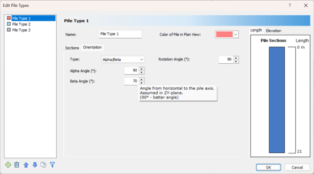
5. Select Pile Types > Pile Type 1 > Orientation and set the Beta angle to 70°

   

   

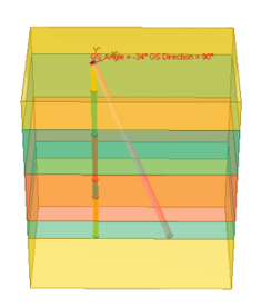
6. In same the same manner as the previous example, enter the global displacements in the X and Z axes:

   Using the angle of the slice base measured in Slide2, resolve the maximum soil displacement to X and Z components

   • |d_x |=|25mm*cos(θ) |
   • |d_z |=|25mm*sin(θ) |
7. Input the Sliding Depth as the L measured from Slide2
8. Change the Ground Slope angle to +34° and direction (bearing in the horizontal plane) to 90°. Click OK
9. As before, Compute the model, open and edit the graphs, and compare the results at the target depth.
10. Click OK to return to the Edit Pile dialog, and then switch back to the Geometry tab.

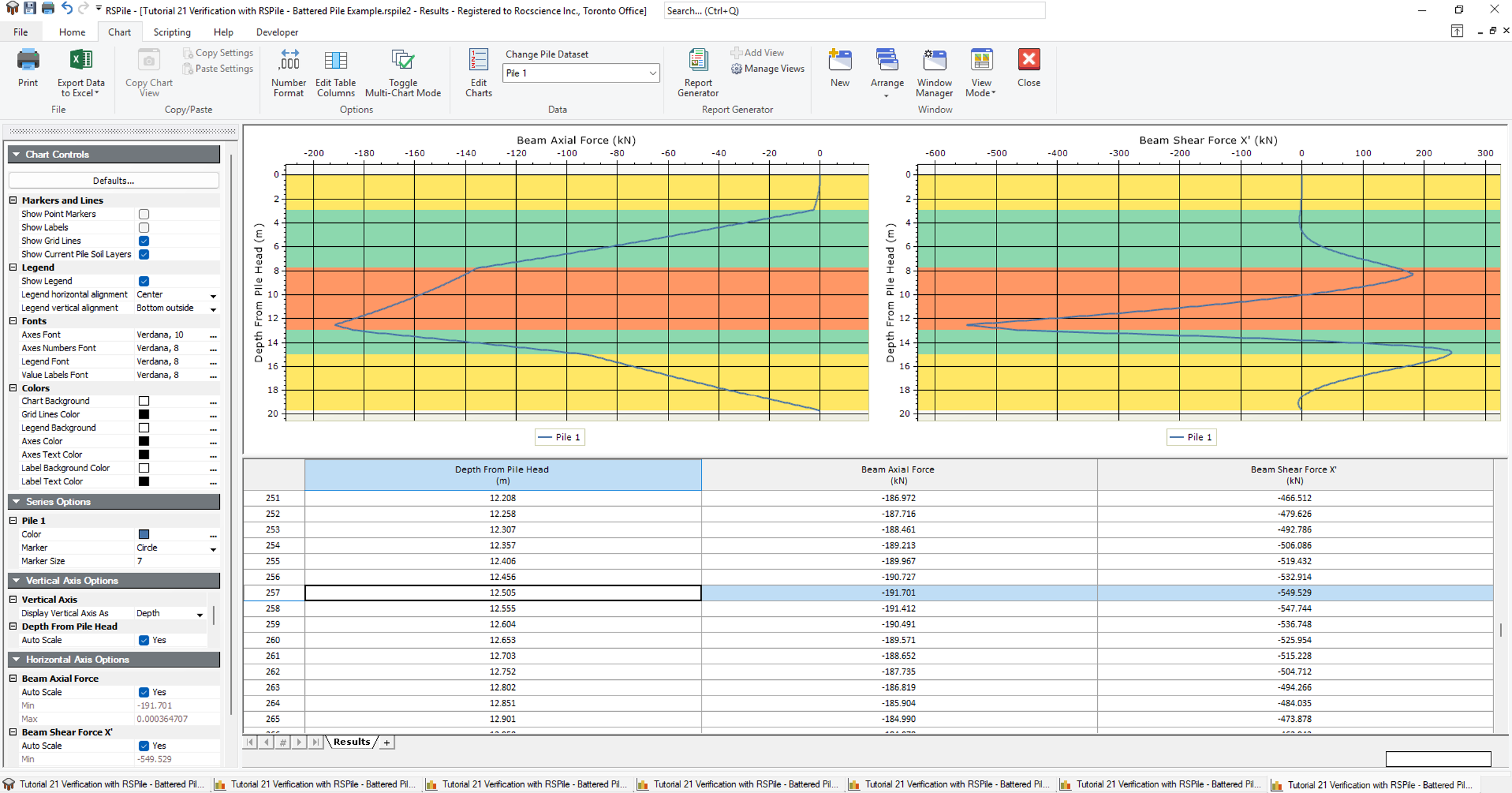
For this example, at a depth of approximately 12.504m, the lateral and axial forces are -549.529kN and -191.701kN respectively.

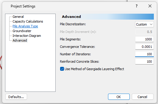
Compared to the resultant force of in Slide2, the results are within acceptable tolerance.  Note that the depth used to get the axial and shear forces from RSPile was not exactly at the desired sliding depth. To achieve a higher level of accuracy, you can increase the number of pile segments in the advanced tab of RSPile’s project settings. 

11. Select Home > Project Settings
12. Select the Advanced tab.
13. Set Pile Discretization to Custom.

14. Set the Pile Segments to 1000.

    

15. Click OK.
16. Select Results > Compute
17. Right-click the pile and select Graph Pile

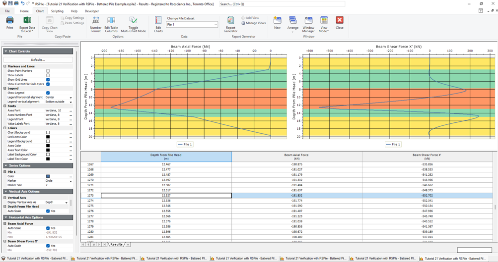
Now, the results tables contains axial and shear forces at finer increments. At 12.527m from the pile head, Fx’ = -552.702kN and Fz’ = -191.832kN respectively. 

This result is even closer to the resultant force displayed in Slide2.

This concludes this tutorial.