12 - Sensitivity Analysis Tutorial

1.0 Introduction

Sensitivity analysis helps geotechnical engineers to identify which input parameters have the most impact on slope stability, and which therefore require the most attention.

In Slide2, any input parameter, which can be defined as a random variable for a probabilistic analysis, can also be specified as a parameter to be varied in a sensitivity analysis.

The Sensitivity Analysis overview page provides helpful information on the topic.

This tutorial will demonstrate how to perform a sensitivity analysis in Slide2. We will generate sensitivity plots for the slope material properties as well as consider the impact of a water table and use the results to identify the input parameters that have the highest influence on factor of safety. As an additional exercise, we will also determine the sensitivity of the slope to seismic coefficient.

Finished Product

The finished product of this tutorial can be found in the Tutorial 12 Sensitivity Analysis.slmd data file. All tutorial files installed with Slide2 can be accessed by selecting File > Recent Folders > Tutorials Folder from the Slide2 main menu.

2.0 Model Geometry

1. Select File > Recent > Tutorials and open Tutorial 12 Sensitivity Analysis – starting file.slmd. (This is the same file used in Tutorial 08 Probabilistic Analysis.)
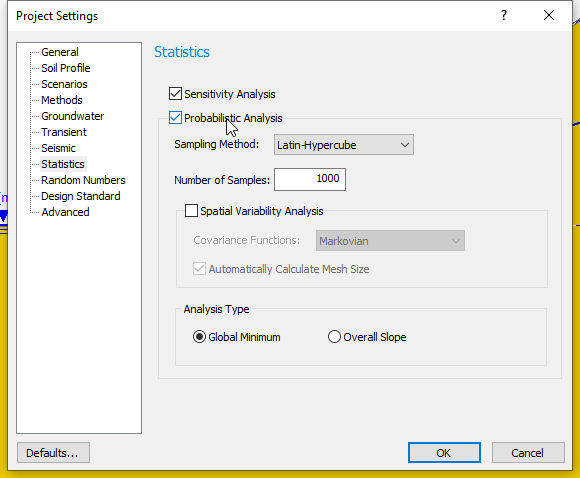
2. Select Analysis > Project Settings
3. Select the Statistics tab and tick the Sensitivity Analysis checkbox as shown below.
   
   
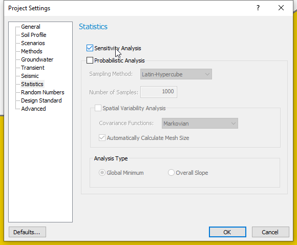
4. Click OK to close the dialog.

3.0 Sensitivity Variables: Material Properties

The procedure for selecting and defining Random Variables for a Sensitivity Analysis is the same as that for Probabilistic Analysis.

However, note that for Sensitivity Analysis:

• Only a Minimum and Maximum value are required for each variable, and no Statistical Distribution or Standard Deviation is required.

1. Select Statistics > Materials to open the Material Statistics dialog.

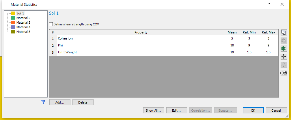
The variables defined for the Probabilistic Analysis in Tutorial 08 are still displayed in the Material Statistics dialog.

Because we are only considering a Sensitivity Analysis, the statistical distribution and standard deviation are no longer displayed in the dialog. Only the mean, minimum and maximum values are needed for the Sensitivity Analysis.

2. Click OK or Cancel to accept the current values and close the dialog.

4.0 Sensitivity Variable: Water Table

We will also consider the sensitivity of the water table location. In Slide2, the Minimum and Maximum locations of a Water Table can be specified on a model by drawing these boundaries or specifying their coordinates using the Prompt line. The program generates a single random variable (a Normalized Elevation ranging between 0 and 1) according to statistical parameters entered in the Water Table Statistics dialog. This random variable is then used to generate Water Table elevations that lie between the Minimum and Maximum boundaries.

To calculate the Mean Water Table, we must specify a Normalized Mean parameter, which will be used to calculate the Mean Water Table boundary. A value of 0.5 indicates a Mean Water Table that is exactly halfway between the Minimum and Maximum levels.

1. Select Statistics > Water Table > Statistical Properties to open the Water Table Statistics dialog.
   
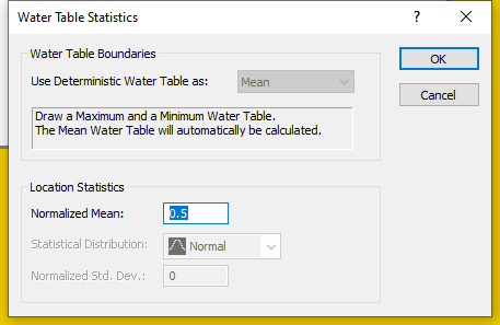
2. We will not change the default Normalized Mean of 0.5.
   The Normalized Mean value is always between 0 and 1.
3. Click OK to close dialog.

We will now draw the Minimum and Maximum Water Table Levels for the model using coordinates. We will first specify the Maximum Water Table level and then the Minimum Water Table locations in the model.

To do this:

1. Select Statistics > Water Table > Draw Max Water Table.
2. With the Prompt line in the status bar activated, enter the following coordinates:
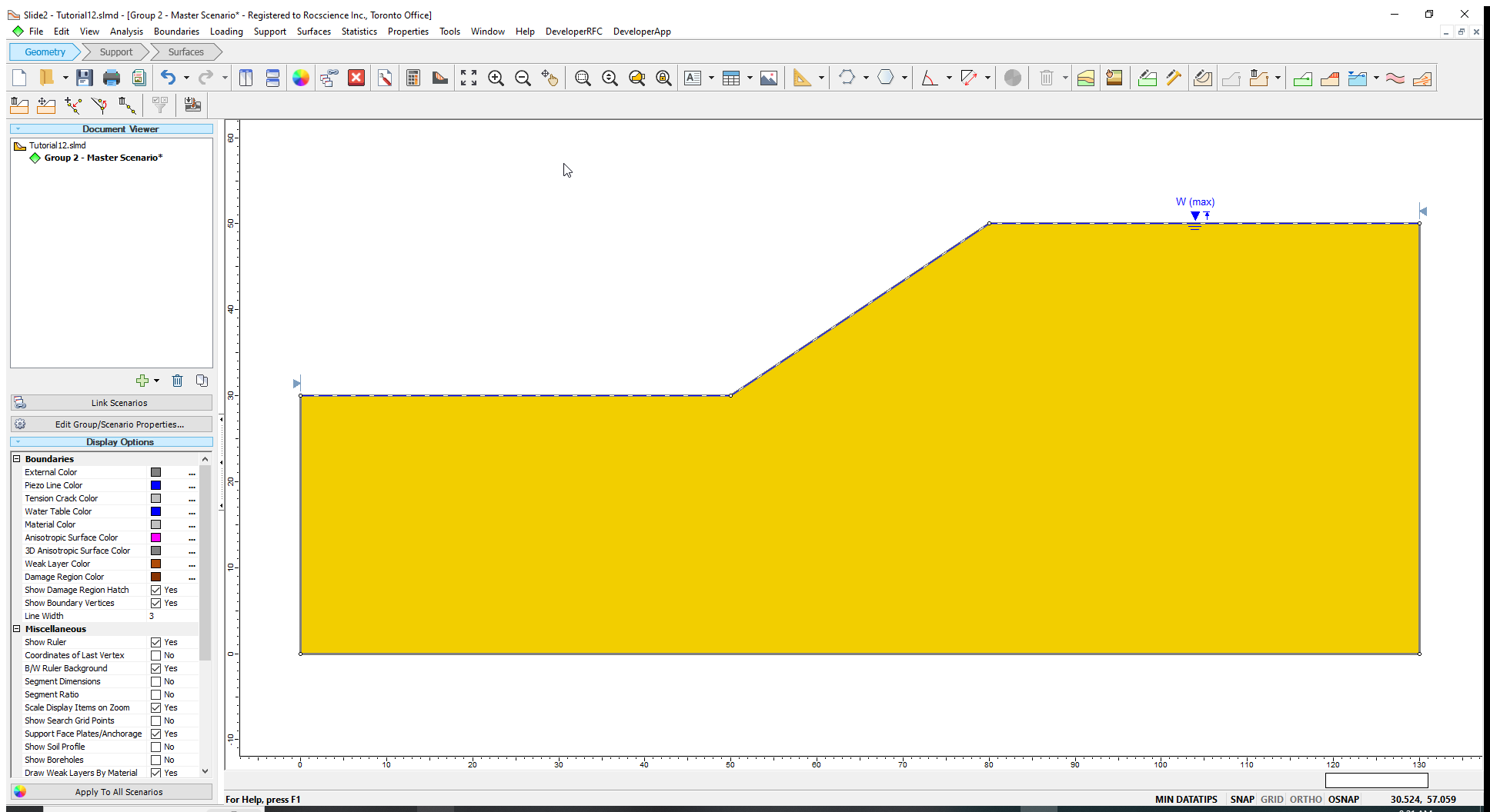
3. (0,30); (50,30) ;(80,50) and (130,50)
4. Press the Enter key or right-click and select Done to finish drawing the maximum water table.

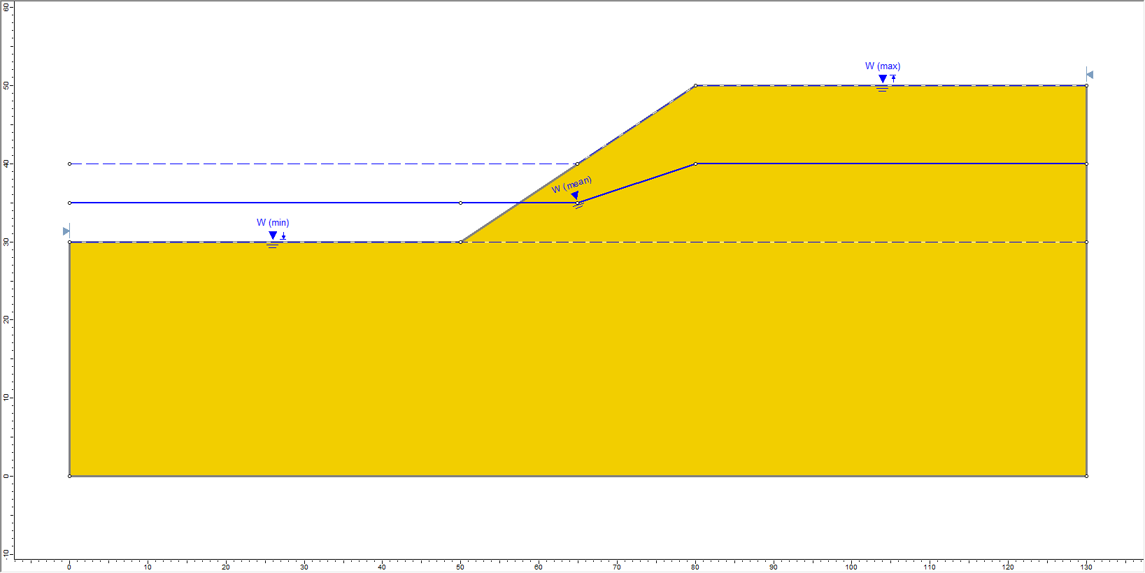
The Maximum Water Table is now shown with a broken line labelled W_(max).

Now let us draw the Minimum Water Table boundary.

1. Select Statistics > Water Table > Draw Min Water Table.
2. Enter the following coordinates in the Prompt line:
   1. (0,30); (50,30) and (130,30).
3. Press the Enter key or right-click and select Done to finish drawing the minimum water table.
4. Select OK to assign the water table to the slope material. (Note that only one material is used in this model.)

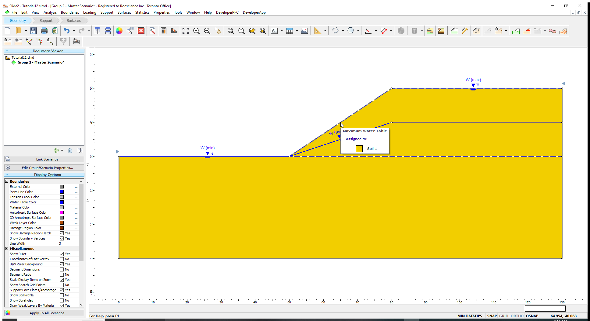
Once the Maximum and Minimum Water Tables are determined, a third water table boundary (i.e., the Mean Water Table) is automatically calculated based on the statistical parameters entered in the Water Table Statistics dialog. This boundary appears on the model, as shown above.

We will now compute the model.

5.0 Computation and Interpretation

1. Select Analysis > Compute to run the analysis.
   
   When running a Sensitivity Analysis with Slide2, the regular (deterministic) analysis is always computed first to determine the Global Minimum slip surface. The Sensitivity Analysis is then performed on the Global Minimum slip surface. This calculation usually takes minimal time; you may not even notice the calculation in the Compute dialog.
   
2. Select Analysis > Interpret to view the results when the computations are done.
   

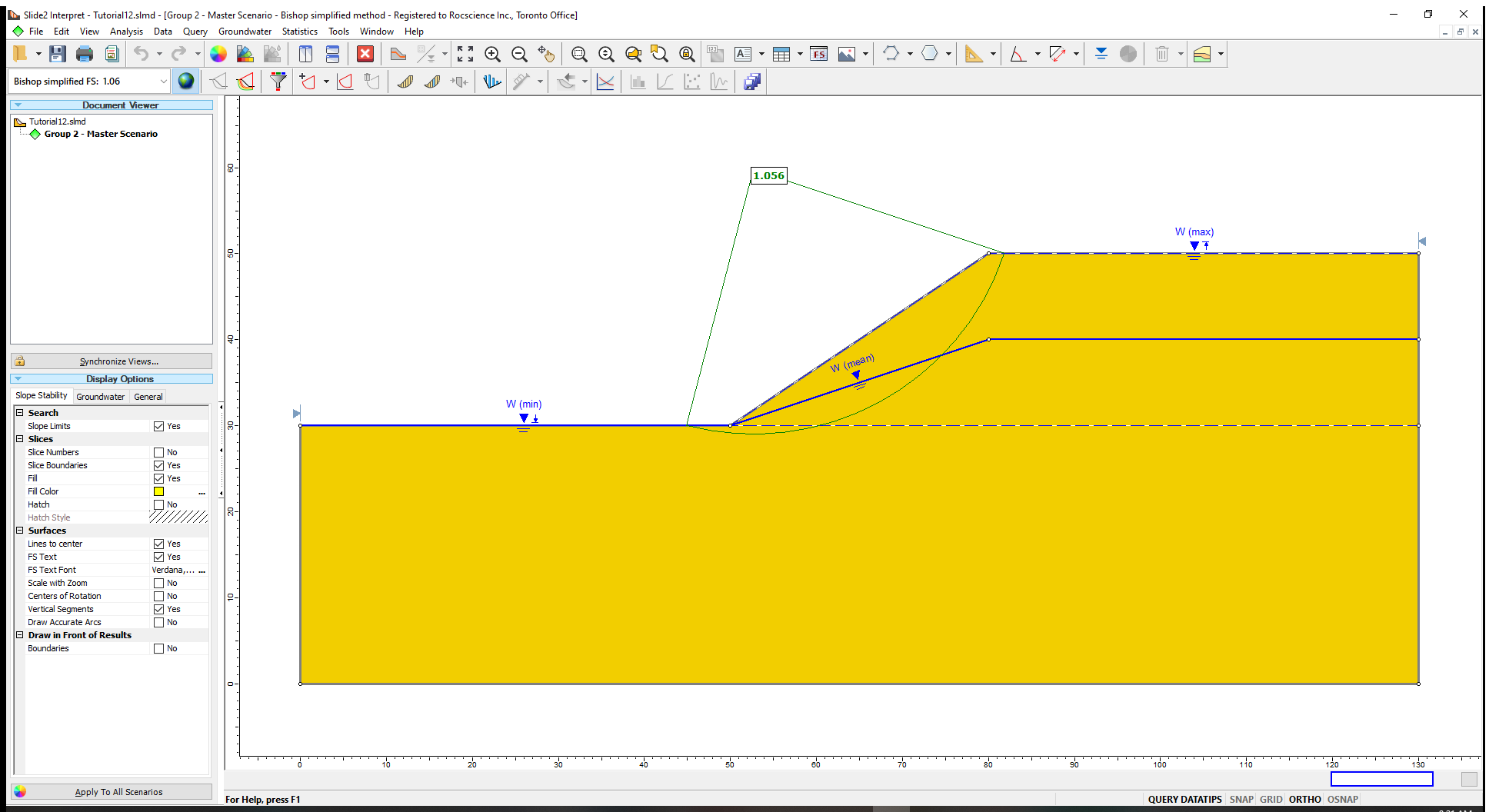
The deterministic safety factor of the Global Minimum slip surface is displayed.

5.1 Sensitivity Plots

To see the Sensitivity Analysis results:

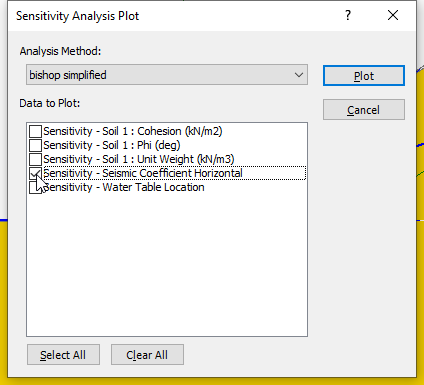
1. Select Statistics > Sensitivity Plot in the Slide2 Interpret window.
   We will plot the sensitivity graphs for the Bishop Simplified method for all the variable properties.
   
2. Click the Select All button to select the checkboxes for the three input parameters selected for sensitivity analysis.
   
3. Click Plot to generate the plots.

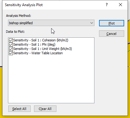
You should see the following sensitivity plot as shown below.

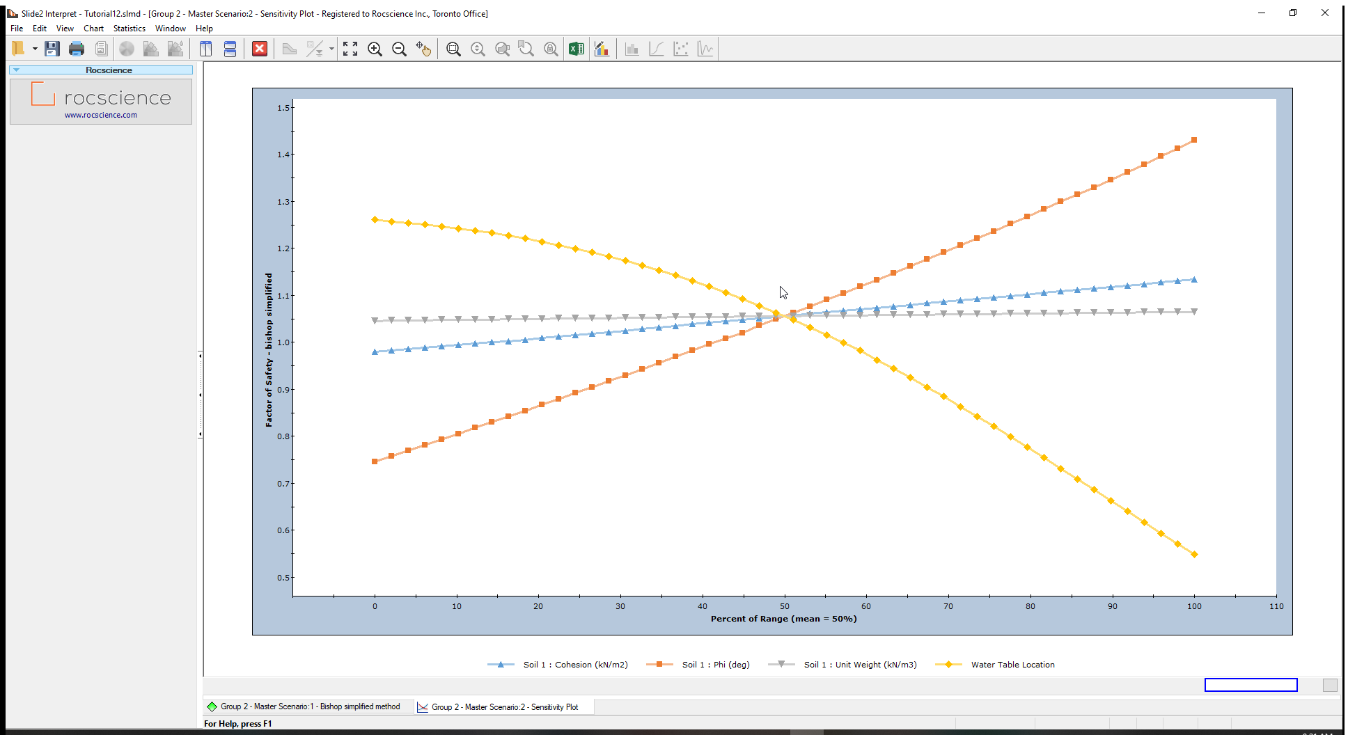
From the sensitivity plot, the line with the steepest slope of the material properties, corresponds to the input parameter, in this case Friction Angle (Phi), which most impacts the factor of safety. This means that the slope’s safety factor is most sensitive to the friction angle. It is least sensitive to the Unit Weight (which has an almost horizontal – near-zero – gradient).

However, the location of the water table is even steeper than the Friction Angle, meaning that it has an even bigger impact on the safety factor, than the material properties. Zero (0) on the x-axis represents the Minimum Water Table boundary, whereas one (1) represents the Maximum Water boundary. Other values determine the relative elevation of the water table (a height along a vertical line) between the Minimum and Maximum boundaries.

All four (4) curves intersect at Percent of Range = 50%. That is the mean value for each variable.

If you would like to see actual parameter values for the horizontal axis, you must plot only one sensitivity variable at a time. (You can do this as an additional exercise.)

5.2 Sampler

You can use the sampler option in Slide2 to determine the value of a parameter that corresponds to a specified safety factor on a sensitivity plot.

For example, you can follow the steps below to determine the critical friction angle, which corresponds to a safety factor of 1.

1. Right-click on the plot, select the Sampler option and Show Sampler.
   
2. The Sampler (dotted crosshair lines) is now displayed on the plot.
3. Move Sampler along the Phi (plot) and locate the point corresponding to the Factor of safety of 1.

6.0 Seismic Coefficient Sensitivity

Let us add one more Sensitivity Analysis variable and re-run the analysis. We will plot a sensitivity graph for a horizontal seismic coefficient.

To do this, return to the Slide2 Model program.

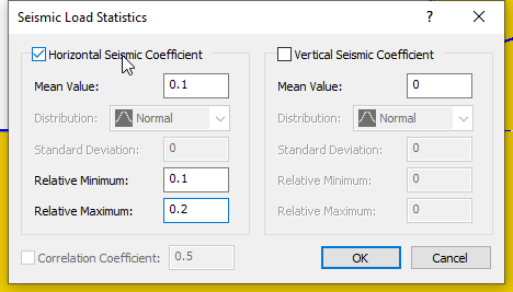
1. Select Statistics > Seismic Load to open the Seismic Load Statistics dialog.
2. In the dialog, tick the checkbox for Horizontal Seismic Coefficient.
3. Enter the following parameters in the following fields.
• Mean Value = 0.1.
• Relative Minimum = 0.1
• Relative Maximum = 0.2.



4. Click OK to close the dialog.
   
   The seismic symbol will be displayed on the model.
   
   
5. Select Analysis > Compute to run the analysis, and then view the results in Interpret when computations are done.
   
6. Create a Sensitivity Plot for only the Horizontal Seismic Coefficient.
   
7. Use the Sampler to determine the critical seismic coefficient corresponding to safety factor = 1.

7.0 Sensitivity and Probabilistic Analysis

A Sensitivity Analysis should not be confused with a Probabilistic Analysis.

Remember:

• A Sensitivity Analysis simply involves the variation of individual variables between the minimum and maximum values. A Sensitivity Analysis is performed on ONLY ONE VARIABLE AT A TIME.
• A Probabilistic Analysis involves the statistical sampling of distributions that you have defined for your random variables. A Probabilistic Analysis uses sampled values of ALL random variables, for each iteration of the Probabilistic Analysis.

However, you can perform BOTH a Sensitivity Analysis AND a Probabilistic Analysis, at the same time, by selecting both checkboxes in Project Settings .

If you do this, note the following:

• The Sensitivity analysis will use the same variables that you have selected for the Probabilistic Analysis.
• The Sensitivity Analysis will only use the Minimum and Maximum values that you have defined for each variable. It will ignore the statistical distributions and standard deviations that you have entered to define the random variables for the Probabilistic Analysis.

This is convenient because if you have already performed a Probabilistic Analysis on a model, then you can also perform a Sensitivity Analysis using all of the same variables, simply by selecting the Sensitivity Analysis checkbox in Project Settings.

This ends the Sensitivity Analysis tutorial.

8.0 Additional Exercises

8.1 Ponded Water / Drawdown Analysis

A variable height of Ponded Water above a slope can also be modelled in a Sensitivity or Probabilistic Water Table analysis with Slide2.

If the Maximum Water Table boundary is located ABOVE the slope at any location, then Ponded water will be automatically created, as necessary, between the Water Table and the slope, in the same manner, as for a regular (Deterministic) Water Table.

Using a Sensitivity Analysis, a drawdown scenario could be quickly analyzed in this manner.

When you define probabilistic Water Table boundaries above a slope, Ponded Water is not graphically displayed on the model, although it will be automatically created and considered during the analysis.

8.2 Tension Crack Statistics

Finally, note that the statistical analysis of a variable Tension Crack boundary, is carried out in the same way as for a Water Table.

In addition, the water level in the Tension Crack can also be specified as a random variable. This is left as an optional exercise for you to experiment with.

For more information, see the Tension Crack Statistics help page.