Strength Type
In the Define Material Properties dialog, a wide variety of Strength Type models are available for modeling shear strength of the various materials of your Slide2 model. Each Strength Type requires various Strength Parameters as described below.
Mohr-Coulomb
The most common way to model soil shear strength is with the Mohr-Coulomb equation:
![]()
where:
s = shear strength
c’ = effective cohesion
![]() = total normal stress
= total normal stress
u = pore pressure
![]() = effective angle of internal friction (phi)
= effective angle of internal friction (phi)
The Mohr-Coulomb equation can be used for either total or effective stress conditions. For a total stress analysis, cohesion and friction angle are defined for total stress conditions. Pore water pressure is not considered, and the Mohr-Coulomb equation is simply:
![]()
Undrained
For the Undrained soil model, the friction angle phi is automatically set to zero. The shear strength is defined only by the cohesion of the material. Three sub-options for defining the Undrained cohesion are available, by selecting from the Cohesion Type drop-down list:
Constant
Cohesion is constant throughout the material.
F(Depth from Top of Layer)
Cohesion is a function of depth, where depth is measured from the top of the material layer that is local to the slice, to the center of a slice base.
![]()
- Cohesion (Top) is the Cohesion at the top of the material layer.
- Cohesion Change is the rate of change of Cohesion with depth.
- If you wish to specify a maximum soil strength, select the Cutoff checkbox and enter a maximum value for Cohesion. If the rate of Cohesion Change is negative, then this value represents the minimum soil strength.
F(Depth from Horizontal Datum)
Cohesion is a function of depth, where depth is measured from a user-specified Datum (y-coordinate) to the center of a slice base.
![]()
- Cohesion (Datum) is the Cohesion at the Datum elevation.
- Cohesion Change is the rate of change of Cohesion with distance (ydatum-y) from the Datum. If the Cohesion Change is positive, then cohesion increases below the datum and decreases above the datum, according to the change in elevation ydatum-y.
- If you wish to specify a maximum soil strength, select the Cutoff checkbox and enter a maximum value for Cohesion. If the rate of Cohesion Change is negative, then this value represents the minimum soil strength.
- Datum is the datum elevation (y-coordinate).
F(Distance to Slope)
Cohesion is a function of depth, where depth is measured from the closest point on the slope (actual distance) to the center of a slice base as shown below.
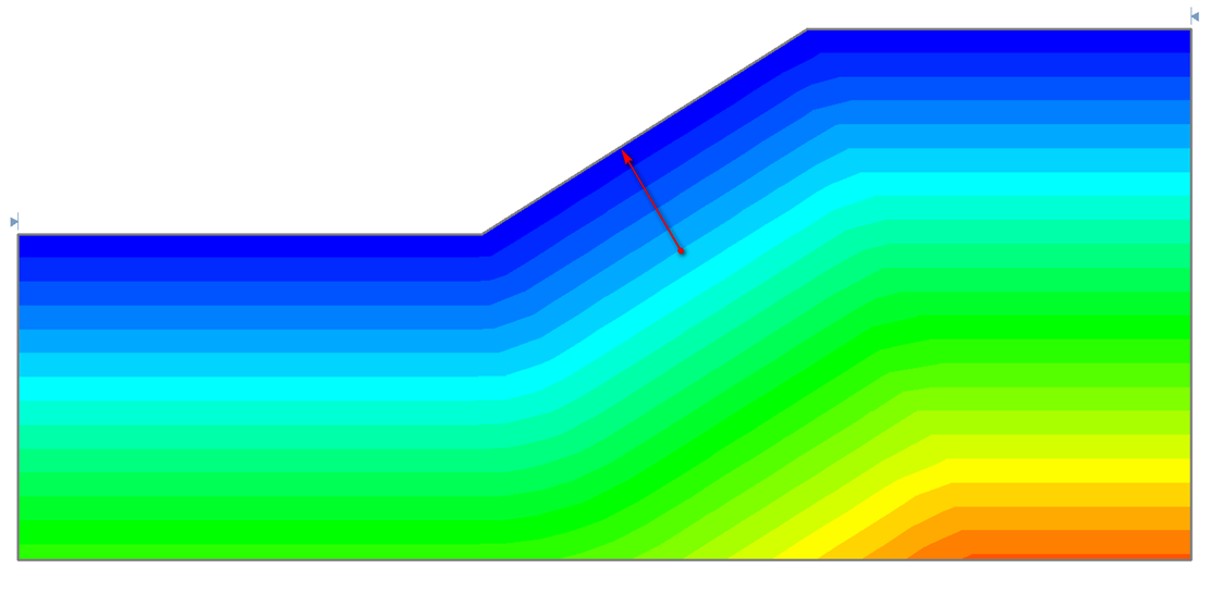
![]()
- Cohesion (Top) is the Cohesion at the top (closest point on the slope) of the slope to the center of a slice base.
- Cohesion Change is the rate of change of Cohesion with depth.
- If you wish to specify a maximum soil strength, select the Cutoff checkbox and enter a maximum value for Cohesion. If the rate of Cohesion Change is negative, then this value represents the minimum soil strength.
Note that the Water Parameters are automatically disabled in the Define Materials dialog when Strength Type = Undrained, since pore water pressure is not required.
No Strength
The No Strength model is intended primarily to model ponded water. When you set the Strength Type = No Strength:
- Strength Parameters are disabled since shear strength is zero (slip surfaces do not pass through a No Strength material). No Strength material contributes only its weight (and hydrostatic force) to the model.
- Water Parameters are not applicable and are disabled.

In most cases, use of the No Strength material is NOT recommended. Ponded water can be modelled in Slide2 much more easily, by simply drawing a Water Table above the External Boundary. See the Add Water Table topic for details. The No Strength material may be useful in some cases if you wish to customize the Unit Weight of Ponded Water (i.e. use a different unit weight from the Pore Fluid Unit Weight specified in Project Settings). Except for this situation, it is recommended that Ponded Water is modelled using a Water Table, rather than the No Strength material.
Infinite Strength
An Infinite Strength material in Slide2 represents a slip surface "exclusion zone", through which slip surfaces are not allowed to pass. Use an Infinite Strength material when you wish to define a region through which a failure surface cannot pass (e.g. a concrete retaining wall, or a heavily reinforced soil region).
For an Infinite Strength material:
- Strength Parameters are disabled.
- Water Parameters are disabled.
"Allow Sliding Along Boundary" - use this option when you have an infinite strength bedrock material at the bottom of your model and want to allow the slip surface to slide along its boundary. This option should otherwise be off.
Anisotropic Strength
The Anisotropic Strength model allows you to define Anisotropic strength properties for a soil or rock mass, by defining cohesion and friction angle along two perpendicular axes. The axes do NOT have to be oriented horizontally and vertically but can be specified at an arbitrary angle as shown in the figure below. Required Strength Parameters are:
- Cohesion 1 and Phi 1 (cohesion and friction angle in 1-direction)
- Cohesion 2 and Phi 2 (cohesion and friction angle in 2-direction, perpendicular to 1-direction)
- Angle (in degrees, measured counter-clockwise from the positive x-axis to the 1-direction)

The cohesion and friction angle for any arbitrary plane is given by:
![]()
![]()
where ![]() = angle between the plane and the 1-direction, as shown in the following figure:
= angle between the plane and the 1-direction, as shown in the following figure:
The Anisotropic Strength model in Slide2 could also be referred to as "Transversely Isotropic" Strength.
Shear / Normal Function
The Shear / Normal Function model allows you to define an arbitrary shear / normal function, to define a non-linear Mohr-Coulomb strength envelope for a material.
When you set the Strength Type to Shear / Normal Function, the Shear / Normal Function drop-list will appear in the Strength Parameters area.
- If there are no Shear / Normal Functions currently defined, this list will be disabled. Select the New button to define a Shear / Normal Function.
- If you have previously defined one (or more) Shear / Normal Functions, then this list will contain the names of the currently defined function(s), and you can simply select an existing function from this list. Or if you need to define a new Shear / Normal Function, select the New button.
- To edit or delete existing Shear / Normal Functions, select the function name from the list, and select the Edit or Delete button.
See the Shear / Normal Strength Function topic for details about defining Shear / Normal Strength Functions.
C / Phi Function
The C / Phi Function model allows you to define an arbitrary c/phi function, to define a non-linear Mohr-Coulomb strength envelope for a material.
When you set the Strength Type to C/Phi Function, the C/Phi Function drop-list will appear in the Strength Parameters area.
- If there are no C/Phi Functions currently defined, this list will be disabled. Select the New button to define a C/Phi Function.
- If you have previously defined one (or more) C/Phi Functions, then this list will contain the names of the currently defined function(s), and you can simply select an existing function from this list. Or if you need to define a new C/Phi Function, select the New button.
- To edit or delete existing C/Phi Functions, select the function name from the list, and select the Edit or Delete button.
See the C/Phi Strength Function topic for details about defining C/Phi Strength Functions.
Anisotropic Function
The Anisotropic Function model is another method for defining Anisotropic strength properties for soil or rock. With this model, you can define discrete angular ranges of slice base inclination, each with its own cohesion and friction angle.
When you set the Strength Type to Anisotropic Function, the Anisotropic Function drop-list will appear in the Strength Parameters area.
- If there are no Anisotropic Functions currently defined, this list will be disabled. Select the New button to define an Anisotropic Function.
- If you have previously defined one (or more) Anisotropic Functions, then this list will contain the names of the currently defined function(s), and you can simply select an existing function from this list. Or if you need to define a new Anisotropic Function, select the New button.
- To edit or delete existing Anisotropic Functions, select the function name from the list, and select the Edit or Delete button.
See the Anisotropic Strength Function topic for details about defining Anisotropic Strength Functions.
Hoek-Brown
The Hoek-Brown strength criterion in Slide2 refers to the ORIGINAL Hoek-Brown failure criterion [ Hoek & Bray (1981) ], described by the following equation:
The original Hoek-Brown criterion has been found to work well for most rocks of good to reasonable quality in which the rock mass strength is controlled by tightly interlocking angular rock pieces.
For lesser quality rock masses, the Generalized Hoek-Brown criterion can be used.
Generalized Hoek-Brown
The Generalized Hoek-Brown strength criterion is described by the following equation:
where:
 is a reduced value (for the rock mass) of the material constant
  (for the intact rock)
 and
and  are constants which depend upon the characteristics of the rock mass
![]() is the uniaxial compressive strength (UCS) of the intact rock pieces
is the uniaxial compressive strength (UCS) of the intact rock pieces
 and
and  are the axial and confining effective principal stresses respectively
See the Generalized Hoek-Brown topic for more information.
Vertical Stress Ratio
With the Vertical Stress Ratio model, the shear strength at the base of each slice is determined by multiplying the effective vertical (overburden) stress by a constant K for the material.
![]()
- The effective vertical stress is computed from the total weight of each slice, and the pore pressure acting at the center of the base of each slice.
- The "vertical stress ratio" K is simply a constant, equal to the ratio of the shear strength to the vertical stress. (e.g. if K = 0.3, then the shear strength will be 30 % of the effective vertical stress.)
Barton-Bandis
The Barton-Bandis strength model can be used to model the shear strength of a joint. The Barton-Bandis strength model establishes the shear strength of a failure plane as:
where ![]() is the residual friction angle of the failure surface [Barton and Choubey, 1977],
is the residual friction angle of the failure surface [Barton and Choubey, 1977],
JRC is the joint roughness coefficient, and JCS is the joint wall compressive strength.
For further information on the shear strength of discontinuities, including a discussion of the Barton-Bandis failure criterion parameters, see Chapter 4 of Practical Rock Engineering by Dr. Evert Hoek, available on the Rocscience website.
Power Curve
The Power Curve model for shear-strength, can be expressed as:
![]()
where:
- a, b and c are parameters typically obtained from a least-squares regression fit of data obtained from small-scale shear tests. The d parameter represents the tensile strength. If included, it must be entered as a positive value.
- If you are using the Power Curve to model the shear strength of a joint, then the parameter
 is the "waviness angle", which is defined as follows:
Waviness Angle
Waviness is a parameter that can be included in calculations of the shear strength of a joint or failure plane. It accounts for the waviness (undulations) of the joint surface, observed over distances on the order of 1 m to 10 m. [ Miller (1988) ] The waviness angle is equal to the AVERAGE dip of a failure plane, minus the MINIMUM dip of the failure plane. A non-zero waviness angle, will always increase the effective shear strength of the failure plane.
If you are NOT modelling the strength of a joint, then you can simply set the waviness angle = 0, and this term in the Power Curve equation will NOT contribute to the shear strength.
Hyperbolic
A Hyperbolic shear strength envelope is defined by the following equation:
![]()
 and
and  in the Hyperbolic shear strength equation. The following figure illustrates a hyperbolic shear strength envelope.
 is defined as the shear strength at
  . is defined as the friction angle at
  .
.The Hyperbolic shear strength model has been found to characterize the shear strength of soil/geo-synthetic interfaces, and other types of interfaces [ Esterhuizen, Filz & Duncan (2001) ]. For example, it could be used to model the shear strength of:
- a concrete/soil interface
- a geotextile/soil interface
You may wish to use the Hyperbolic shear strength model, to model the failure mode of "direct sliding" along a Geosynthetic/Soil interface. In this case, you will have to define a narrow layer of soil along the geotextile, and assign a material type which uses the Hyperbolic shear strength model.
Discrete Function
The Discrete Function option allows you to specify the shear strength at discrete x,y locations throughout a material. The shear strength at any point within the material can then be interpolated. Shear strength may be specified for either the undrained case (cohesion only), or drained (cohesion and friction angle).
When you set the Strength Type to Discrete Function, the Discrete Function drop-list will appear in the Strength Parameters area.
- If there are no Discrete Functions currently defined, this list will be disabled. Select the New button to define a Discrete Function.
- If you have previously defined one (or more) Discrete Functions, then this list will contain the names of the currently defined function(s), and you can simply select an existing function from this list. Or if you need to define a new Discrete Function, select the New button.
- To edit or delete existing Discrete Functions, select the function name from the list, and select the Edit or Delete button.
See the Discrete Strength Function topic for details about defining Discrete Strength Functions.
Drained-Undrained
The Drained-Undrained option allows you to define a soil strength envelope which considers both drained and undrained Mohr-Coulomb strength parameters. The shear strength is defined in terms of effective stress parameters c’ and phi’, up to a maximum value of shear strength defined by the undrained cohesion Cu.
If you only need to define constant strength parameters which do NOT vary with depth, then you can enter the parameters directly in the Define Materials dialog. In this case, the shear strength envelope is defined by constant values of:
- Cu (undrained cohesion)
- c’/Cu ratio (drained cohesion c’ is defined as a fraction of Cu)
- drained phi’
Cohesion Varies with Depth
If the cohesion is variable with depth, then you must select the Cohesion varies with depth checkbox. This will enable the Define button. Select the Define button, and you will see another dialog (the Drained-Undrained Strength Properties dialog), in which you can define the drained and/or undrained cohesion as a function of depth.
See the Drained-Undrained Strength topic for more information.
Undrained / Vertical Stress Function
With the Undrained / Vertical Stress model allows you to define an undrained shear / vertical stress strength envelope for a material.
When you set the Strength Type to Undrained / Vertical Stress Function, the Undrained / Vertical Stress Function drop-list will appear in the grid area.
- If there are no Undrained / Vertical Stress Functions currently defined, this list will be disabled. Select the Edit button to define an Undrained / Vertical Stress Function.
- If you have previously defined one (or more) Undrained / Vertical Functions, then this list will contain the names of the currently defined function(s), and you can simply select an existing function from this list. Or if you need to define a new Undrained / Vertical Function, select the Edit button.
- To edit or delete existing Undrained / Vertical Functions, select Edit button.
See the Undrained / Vertical Stress topic for more information
Anisotropic Linear
The Anisotropic Linear strength model (Mercer, 2012; Mercer, 2013), is similar to the Anisotropic Strength model described above. It allows you to define a material with the following anisotropic strength characteristics:
- Bedding plane cohesion and friction angle
- Rock mass cohesion and friction angle
- Angle of bedding plane from horizontal
- Parameters A and B which define a linear transition from bedding plane strength to rock mass strength, with respect to shear plane orientation.
See the Anisotropic Linear Strength Function topic for details.
Generalized Anisotropic
The Generalized Anisotropic Strength option allows you to create a composite strength model, in which you can assign any strength model in Slide2, to any range of slice base orientations. For example, you could create a material with Hoek-Brown properties over a range of orientations, and Mohr-Coulomb properties over another range of orientations (e.g. to simulate a weak bedding orientation in a rock mass).
See the Generalized Anisotropic topic for details.
Snowden Modified Anisotropic Linear
The Snowden Modified Anisotropic Linear strength model (Mercer, 2013) is based on the Anisotropic Linear strength model, with the following additions:
- allows you to define non-linear stress-dependent strength envelopes for the rock mass and bedding material, and
- allows non-symmetric anisotropy.
See the Snowden Modified Anisotropic Linear topic for details.
SHANSEP
The SHANSEP model (Stress History and Normalized Soil Engineering Properties) is widely used for modelling the undrained shear strength of soils (Ladd and Foote, 1974).
See the SHANSEP strength topic for details.
CNI
The CNI strength model in Slide2 uses the non-linear formulation [Cylwik et al., 2023] described by the following equation:
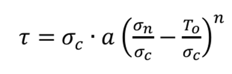
where:
σc is the rock mass compressive strength
a is the strength magnitude coefficient
σn is the normal stress
To is the direct tensile strength expressed as a negative value
n is the curvature coefficient
See the CNI topic for more detailed information.