Analysis of Triaxial Lab Data
1.0 Introduction
This tutorial will involve fitting two strength models to a triaxial lab dataset for intact rock.
• Generalized Hoek-Brown
• Mohr-Coulomb
Finished Product:
The finished product of this tutorial can be found in the Tutorial 3.rsdata data file. All tutorial files installed with RSData can be accessed by selecting File > Recent Folders > Tutorials Folder from the RSData main menu.
2.0 Creating model
- Open RSData.
- Select the Rock template for Project template and click OK.
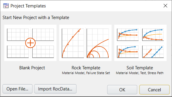
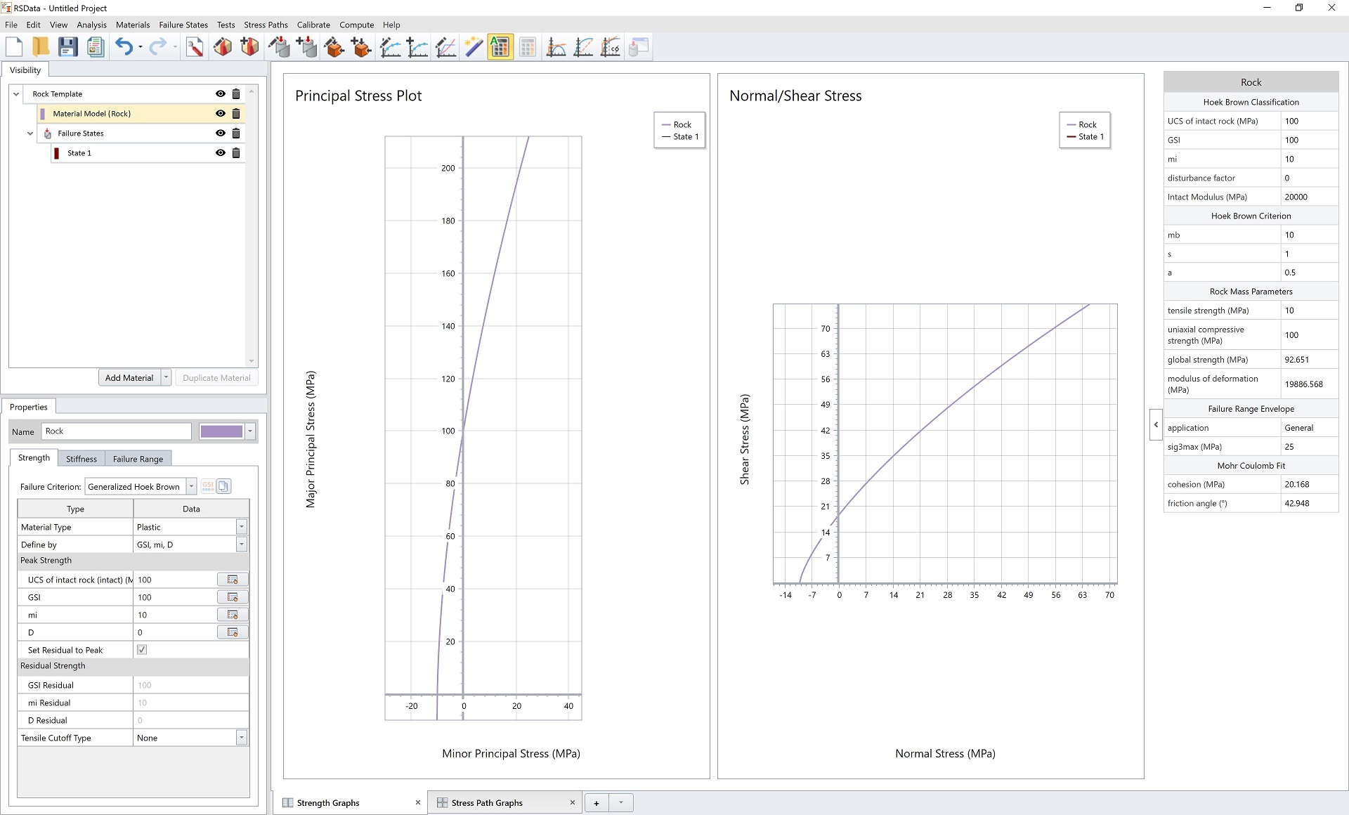
By default, strength graphs are presented, and a rock template is given for Rock Project Template. Within the rock template, a rock material model and an empty failure state are included. The rock material is also depicted on the strength graphs.
There is one thing worth noticing before starting. Let’s check the Rock’s properties.
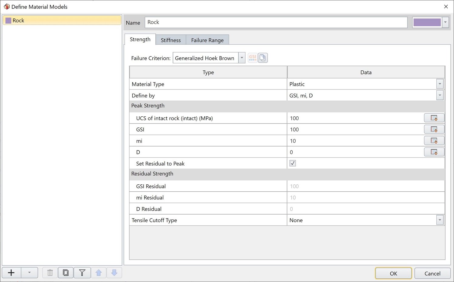
Select  Define Material Model.
In the Define Material Models dialog, select the Rock model on the left side. Notice here are the default parameters for rock as shown below. The Strength and Failure Range parameters will be updated later after calibration.
3.0 Failure State
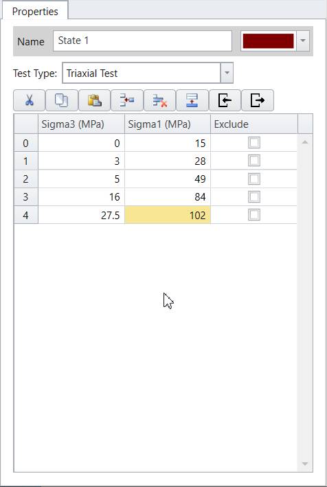
- In the Visibility Tree, select State 1.
- In the Properties Pane below, select Test Type = Triaxial Test.
- Enter the following triaxial data points in the data grid:
| Sigma3 (MPa) | Sigma1 (MPa) |
| 0 | 15 |
| 3 | 28 |
| 5 | 49 |
| 16 | 84 |
| 27.5 | 102 |
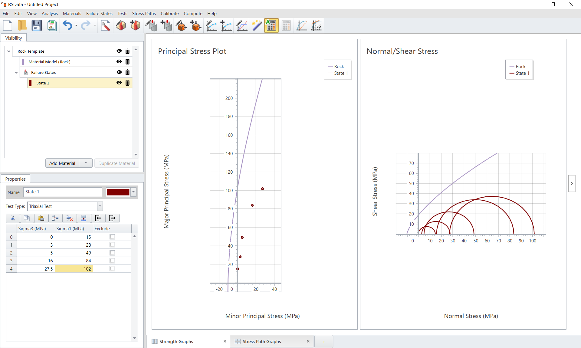
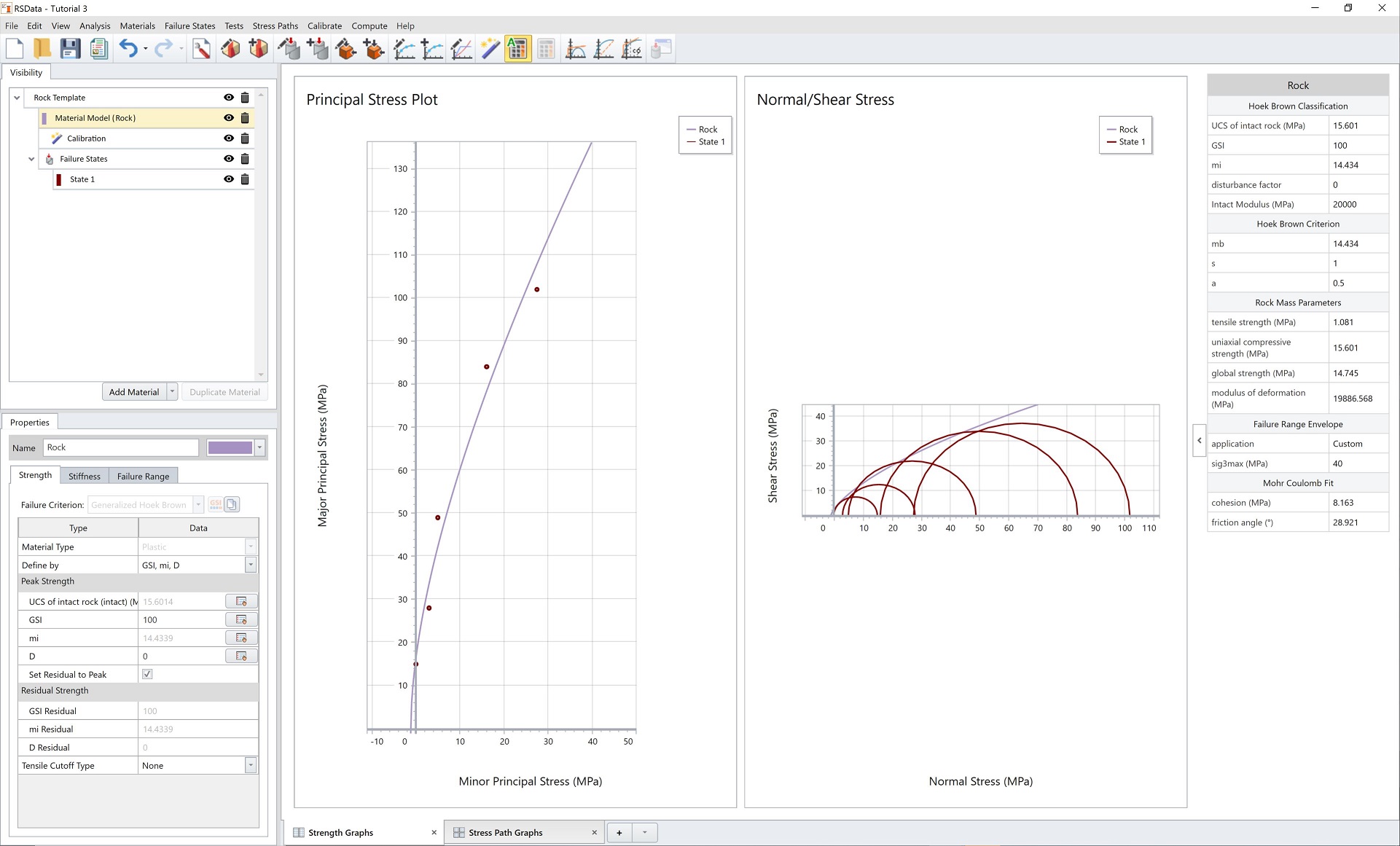
Triaxial data points are drawn as points on the Principal Stress Plot representing the failures and as Mohr circles on the Normal vs. Shear Stress graphs as follows:
4.0 Calibration and Results– Generalized Hoek-Brown
The next step is to curve fit/calibrate the dataset and find the best fit failure envelopes with Generalized Hoek-Brown method.
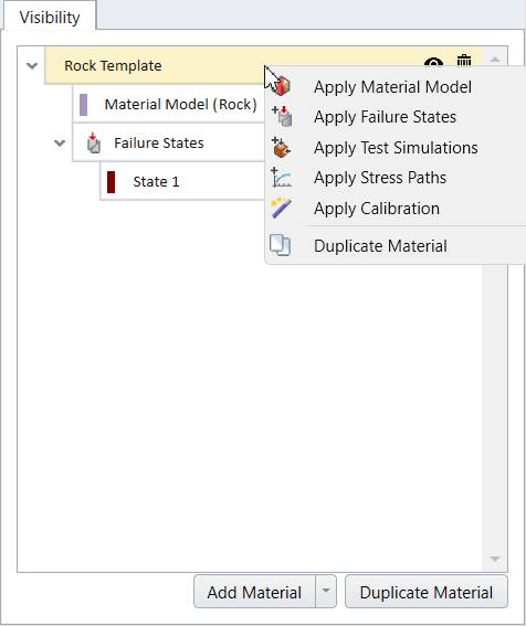
- Under the Visibility Tree, right click on Rock Template, and select Apply Calibration.
- A Calibration set is added to the Rock Template. Select the added Calibration set.
- In the properties section below, enter the following parameters in order:
- Algorithm = Modified Cuckoo
- Error Summation = Basic
- Error Type = Absolute
- Leave other setting as default. The properties section will display as follows:
- By default the
 Auto Compute is selected and the results will be updated. The user has control to toggle the Auto Compute on and off.
 - Select Define Material Model.
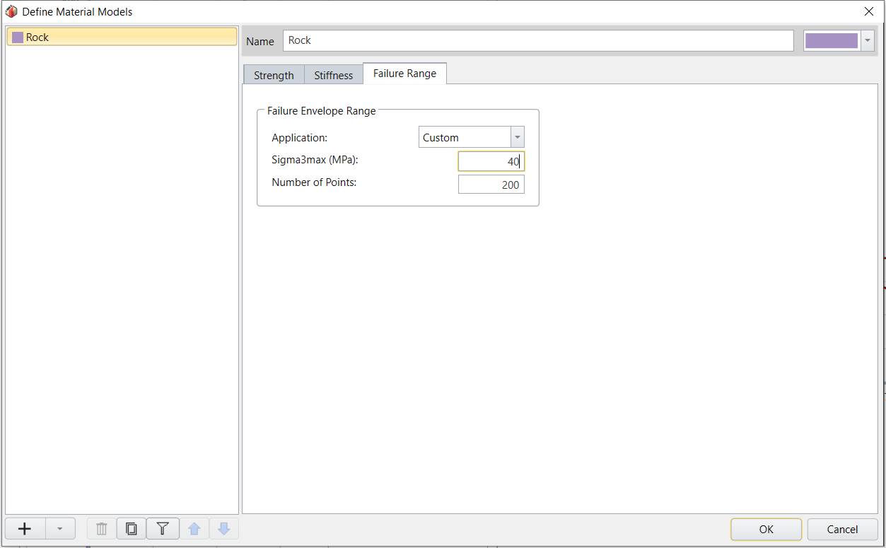
- Change the Application to Custom and then set the Range to 40 MPa.
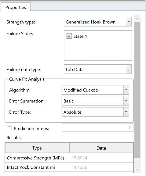
Note: By default, Generalized Hoek Brown is used as the Calibration Strength Type in this tutorial. Failure data type is set to Lab Data, which is subjected to the lab data points in Failure State 1.
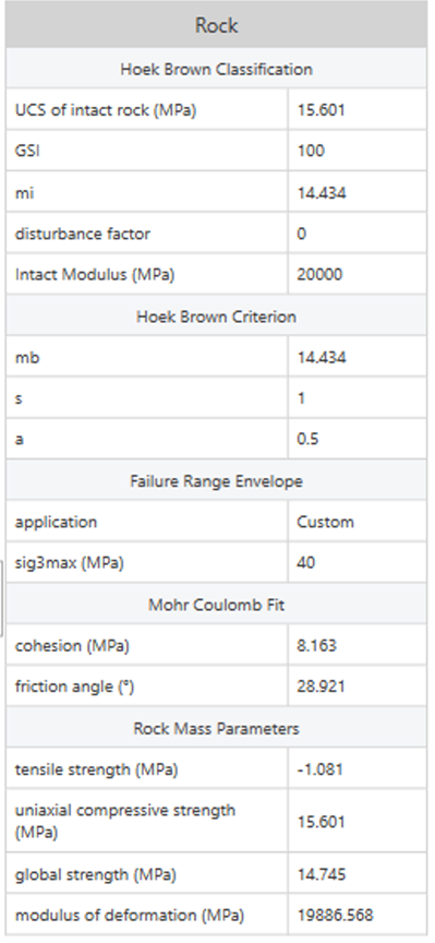
The calibrated results are presented in the table on the Properties of the Calibration node and also in the collapsible chart on right side panel. Here, the calculated Compressive Strength is 15.60 MPa, Intact Rock Constant mi is 14.43, and Residuals is 146.085. These results will also be updated to the material parameters.
For the Strength tab, Peak Strength parameters and Residual Strength parameters are calculated and updated. 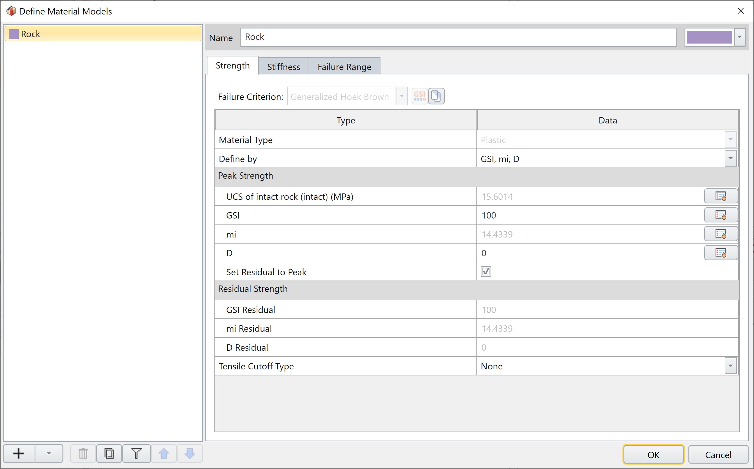
In the Failure Range tab, the Sigma3max value can be updated.
This will update the failure envelop plot and affect the Mohr Coulomb Fit and Rock Mass Parameters that are calculated in the right hand side table.
Click OK to close the dialog.
Now let’s look at the curve fitting failure envelopes. The purple line in both plots are the calibrated envelopes as shown below. We can double click on the plot to get bigger views.
5.0 Calibration and Results– Mohr Coulomb
In this section we will calibrate with Mohr Coulomb method.
- Select
 Calibrate from the toolbar at the top.
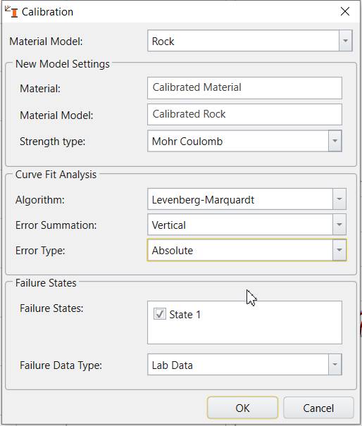
 - In the Calibration dialog, enter the following parameters in order:
- Calibration Strength type = Mohr Coulomb
- Select the checkbox beside “State 1”
- In the Curve Fit Analysis section:
- Algorithm = Levenberg-Marquardt
- Error Summation = Vertical
- Error Type = Absolute
- Click OK to save and close the dialog.
The dialog should look as follows:
A new material is created, and the Mohr Coulomb calibration is applied to it.
The new calibration should Auto compute. If not, click the  Compute icon to compute the calibration.
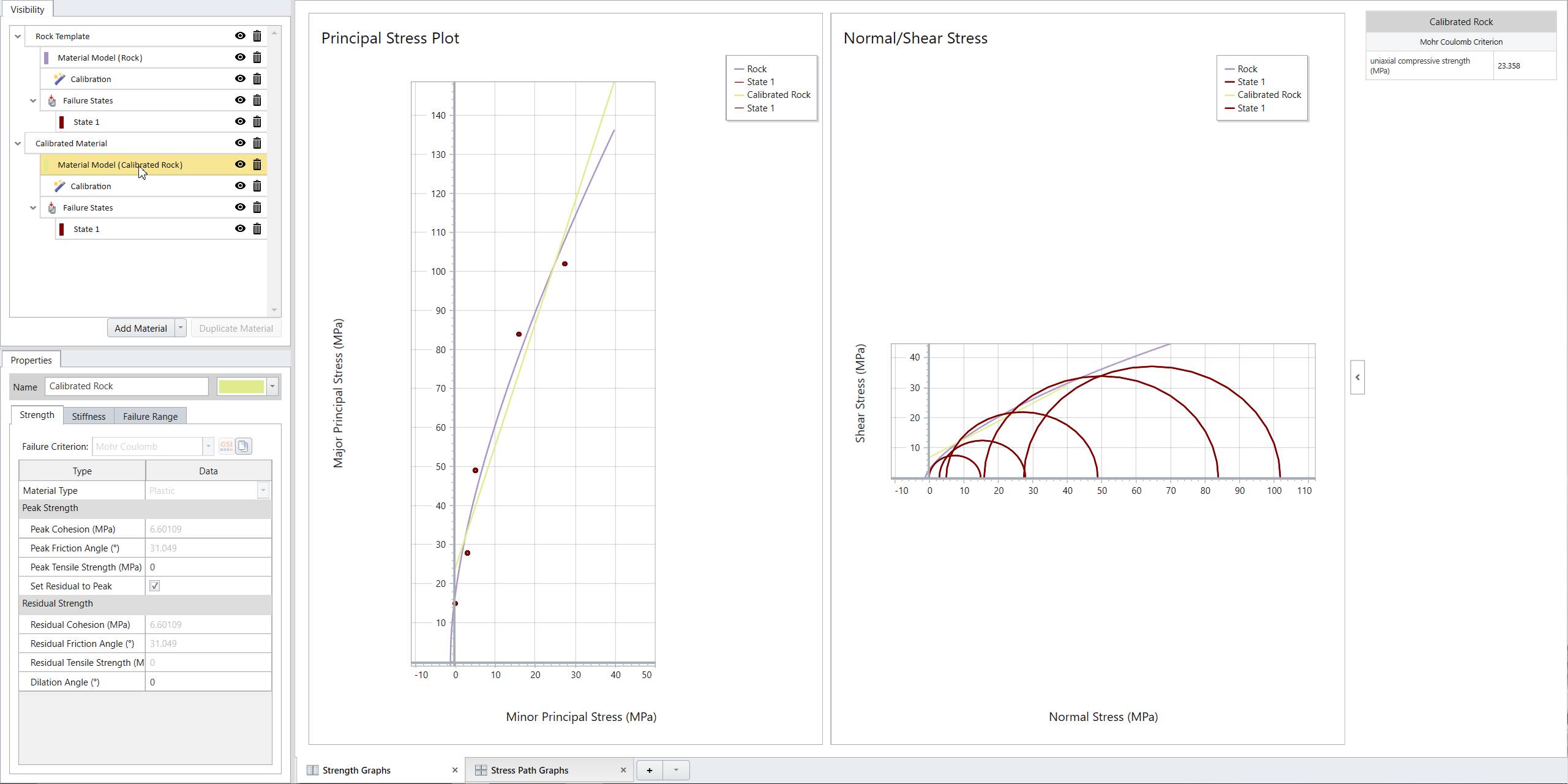
The Mohr Coulomb method calibration results are displayed in results table at the bottom of properties tab, and on Principal Stress Plot and Normal vs. Shear Stress plots as light green lines as shown below.
The results are also updated to the material properties of Material Model 1.
5.1 ADJUSTING THE FAILURE ENVELOPE RANGE
In the Strength Graphs, the calibrated failure envelopes for both methods are difficult to see. We can adjust the Failure Envelope Range to get a better view.
- Under the visibility tree, select Material Model (Calibrated Rock).
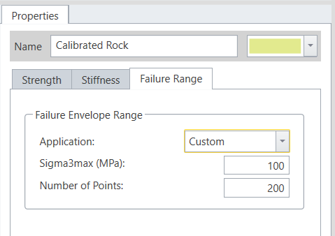
- In the Properties pane, select the Failure Range tab.
- Enter the following:
- Application = Custom
- Sigma3max (MPa) = 100
- Leave other settings as default.
Note: the sigma3max is set to 100 MPa because the largest normal stress in Mohr Circle is 100 MPa.
Now, the maximum minor principle stress (sigma3max) has been increased to 100 MPa. The calibrated failure envelopes are updated as follows:
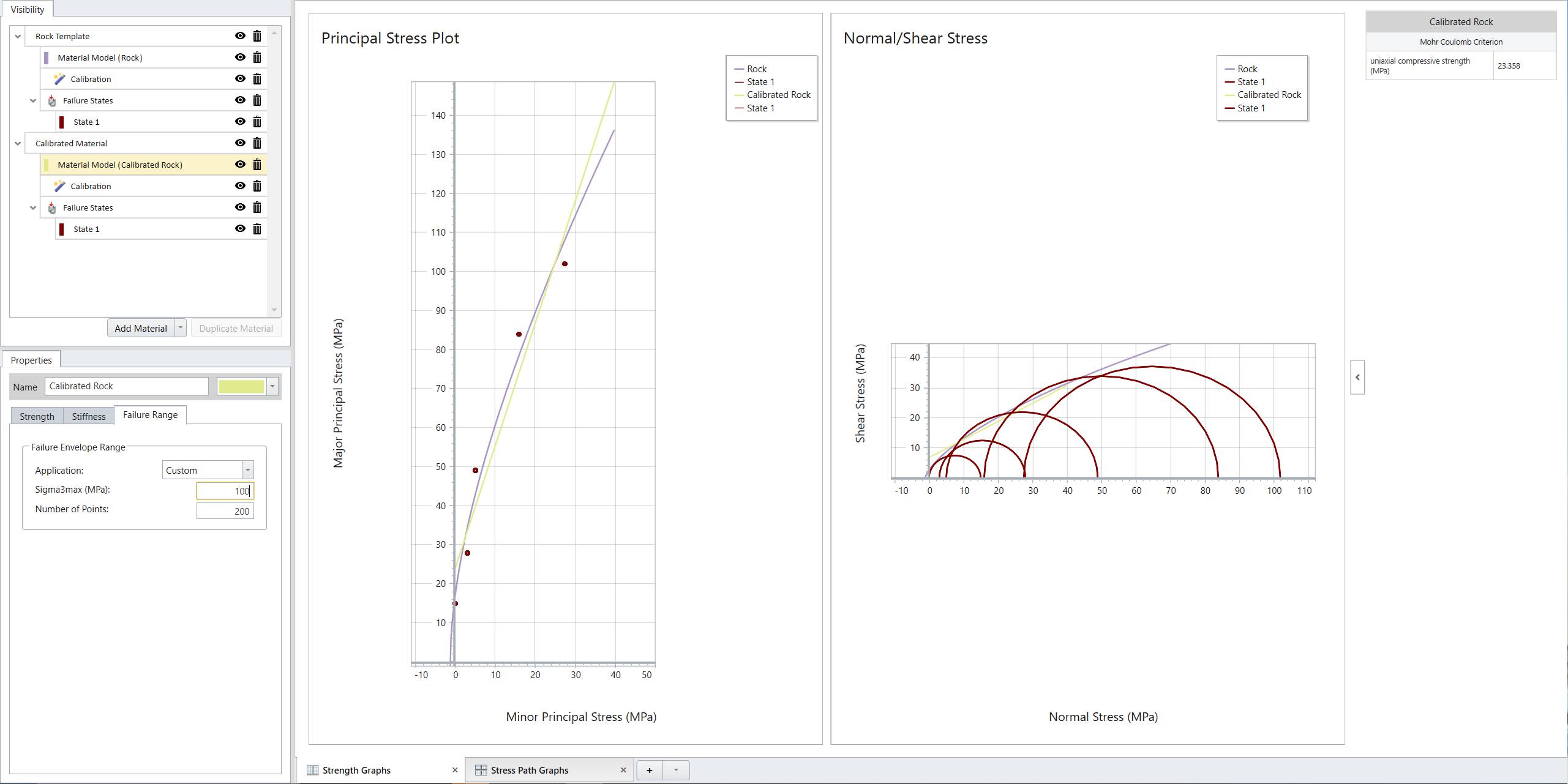
Now we can compare calibration results between Generalized Hoek-Brown method and Mohr Coulomb method both graphically and numerically.
Here concludes RSData tutorial – Analysis of Triaxial Lab Data.