RS3 Quick Start
1.0 Introduction
This tutorial introduces some of the basic features of RS3. The model used in this tutorial analyzes the effect of a foundation being constructed near a sloped underground tunnel. We will create a multi-stage model using stages so that we may observe how the soil behaves at each specific step of the foundation's construction and compare the results. The stages that will be considered are:
- Initial Conditions
- Excavate Tunnel
- Excavate Foundation
- Pour Concrete Foundation
- Loading Foundation
2.0 Starting a Model
Open RS3. You will see a blank workspace.
- Select: Analysis > Project Settings

Our first step is to configure the analysis parameters for the model. Always check that you are working with the right units.
Units
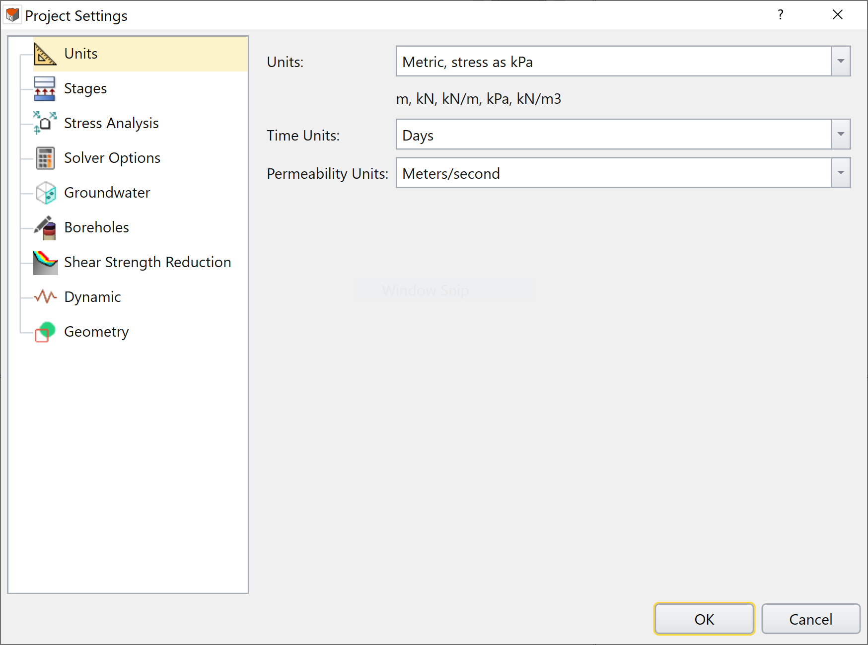
- Select the [Units] tab.
- Set Units to Metric, stress as kPa and keep everything else as default. The dialog should look as shown below:
Now we will be adding additional Stages to our analysis.
Stages
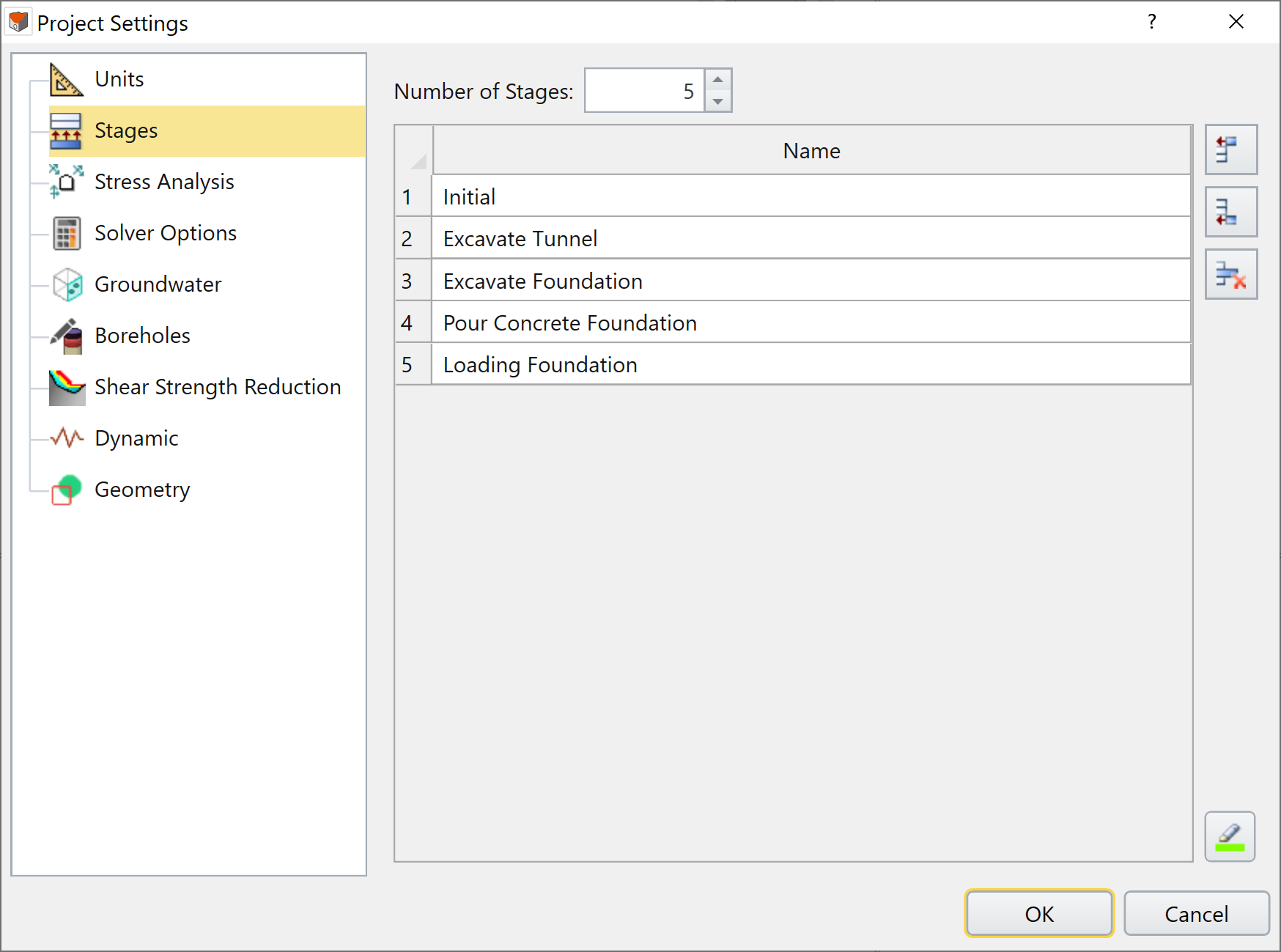
- Select the [Stages] tab. Enter Number of Stages = 5 and input each stage name as shown in the table below:
Stages | Stage Name |
1 | Initial |
2 | Excavate Tunnel |
3 | Excavate Foundation |
4 | Pour Concrete Foundation |
5 | Loading Foundation |
After inputting the stage names, the dialog should look as follows:
For this model, we will NOT be including any groundwater in the analysis so we must indicate this in the project settings.
Groundwater
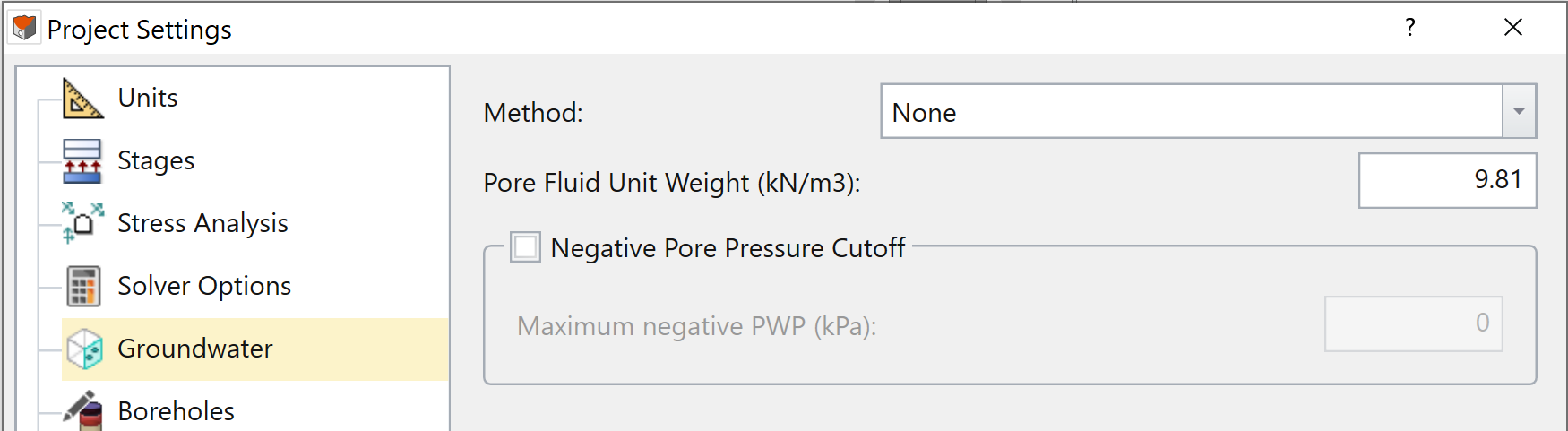
- Select the [Groundwater] tab. By default the Method is set to Phreatic Surfaces. Change Method to None.
- Click OK to save and close the project settings dialog.
The dialog should look as follows:
3.0 Defining the Materials
RS3 is designed with an intuitive workflow to help guide the user through the required steps in creating a model. Under each tab, the toolbars and menus are customized to provide the user with the functions they will need in each step of creating their model.
- We will begin with the Geology workflow tab

- Select: Materials > Define Materials

- Enter the following properties for “Material 1” and “Material 2” in the [Initial Conditions] and [Stiffness] tab. Leave the other options with default settings.
- Select OK to save and close the Material Properties dialog.
The Define Materials dialog has several tabs that are used to assign different material properties.
Name | Initial Loading | Unit Weight (kN/m3) | Young's Modulus (kPa) | Poisson's Ratio | |
Material 1 | Soil | Field Stress & Body Force | 20 | 20000 | 0.3 |
Material 2 | Concrete | Body Force Only | 27 | 280000 | 0.3 |
The Material Properties dialog for Soil should look like the following:

4.0 Creating Geometry
Ensure the Geology workflow tab is still selected from the workflow.
- Select: Geometry > Create External Box

- A Create External dialog will open. Enter:
- First Corner (x, y, z) = (0, 0, 0)
- Second Corner (x, y, z) = (30, 30, -20)
- Click OK.

- The external volume geometry should now be displayed in the viewports. Under the visibility pane on the left, select the 'External' volume and re-name it to 'Soil' using properties pane below. Your screen should look like the following:

5.0 Excavation
- Select the Excavations workflow tab

5.1 CREATING A CYLINDER FOR THE UNDERGROUND TUNNEL
We will now define a cylinder to represent the underground tunnel.
- Select: Geometry > 3D Primitive Geometry > Cylinder

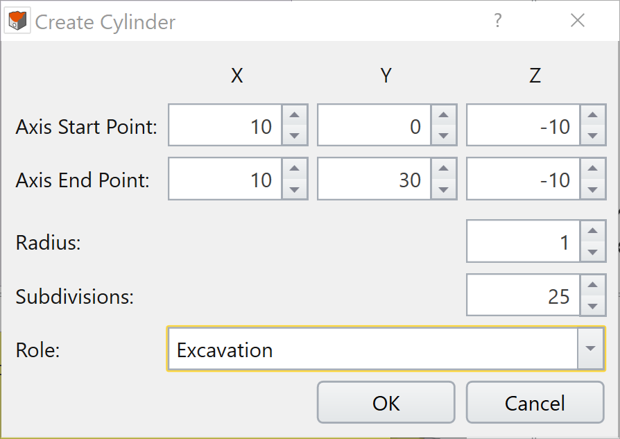
- Enter the following axis and properties:
- Axis Start Point (x, y, z) = (10, 0, -10),
- Axis End Point (x, y, z) = (10, 30, -10),
- Radius = 1
- Subdivisions = 25
- Role = Excavation
- Click OK to save and close the dialog.
The model should now look like the following:

Next, we are going to represent the foundation by creating an extruded circular polyline.
5.2 EXTRUDING A CIRCLE FOR THE FOUNDATION
- Select: Geometry > Polyline Tools > Draw Polyline
 . A Draw Polyline pane will open on the left side of the screen.
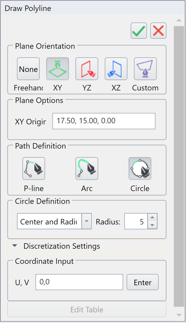
- Set Plane Orientation = XY
- Now input the following:
- XY Origin (x, y, z) = (17.5, 15, 0)
- Path Definition = Circle
- Circle Definition = Center and Radius
- Radius = 5
- Coordinate Input U, V = 0, 0. Press Enter.
- Click the green checkmark
 located at the top-right corner to close the pane.
The model should look as shown below:

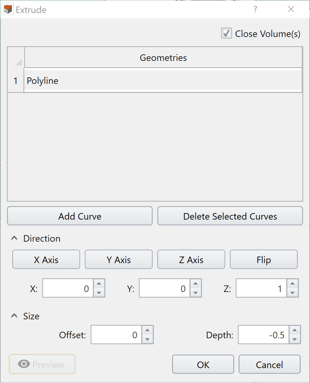
- Select Polyline in the visibility pane.
- Select: Geometry > Extrude/Sweep/Loft Tools > Extrude

An Extrude Geometry dialog will appear as shown below.
- Under Direction keep (x, y, z) = (0, 0, 1) and change Depth = -0.5.
- Click OK.
The other entities (Cylinder and Polyline_extruded) in the visibility pane are geometry objects that are currently not interacting with the external volume.

In order to integrate these objects into the external volume of the model, we need to use the Divide All Geometry function to convert the geometry objects to sub-volumes in the main model.
5.2.1 Divide All Geometry
Now that we’ve defined the external box and the objects to be cut into it, we can use the Divide All Geometry function.
- Select: Geometry > 3D Boolean > Divide All Geometry

The Divide All Parameters dialog helps users to fine-tune the behaviour of the Divide All function. Setting Quality to the Default option is suitable for a wide range of models in general, however, there are cases where changing the setting is required to successfully intersect every geometry with the external volume.
For more detail about each option under Divide All Parameters, please refer to Divide / Un-Divide All Geometry.
- We will keep everything default for now.
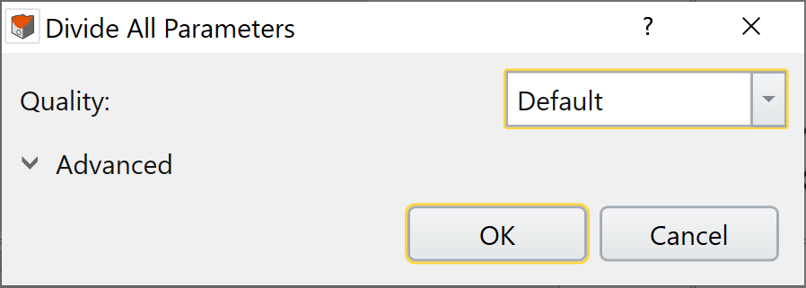
- Click OK to begin dividing.
Your model should now look similar to the one below.
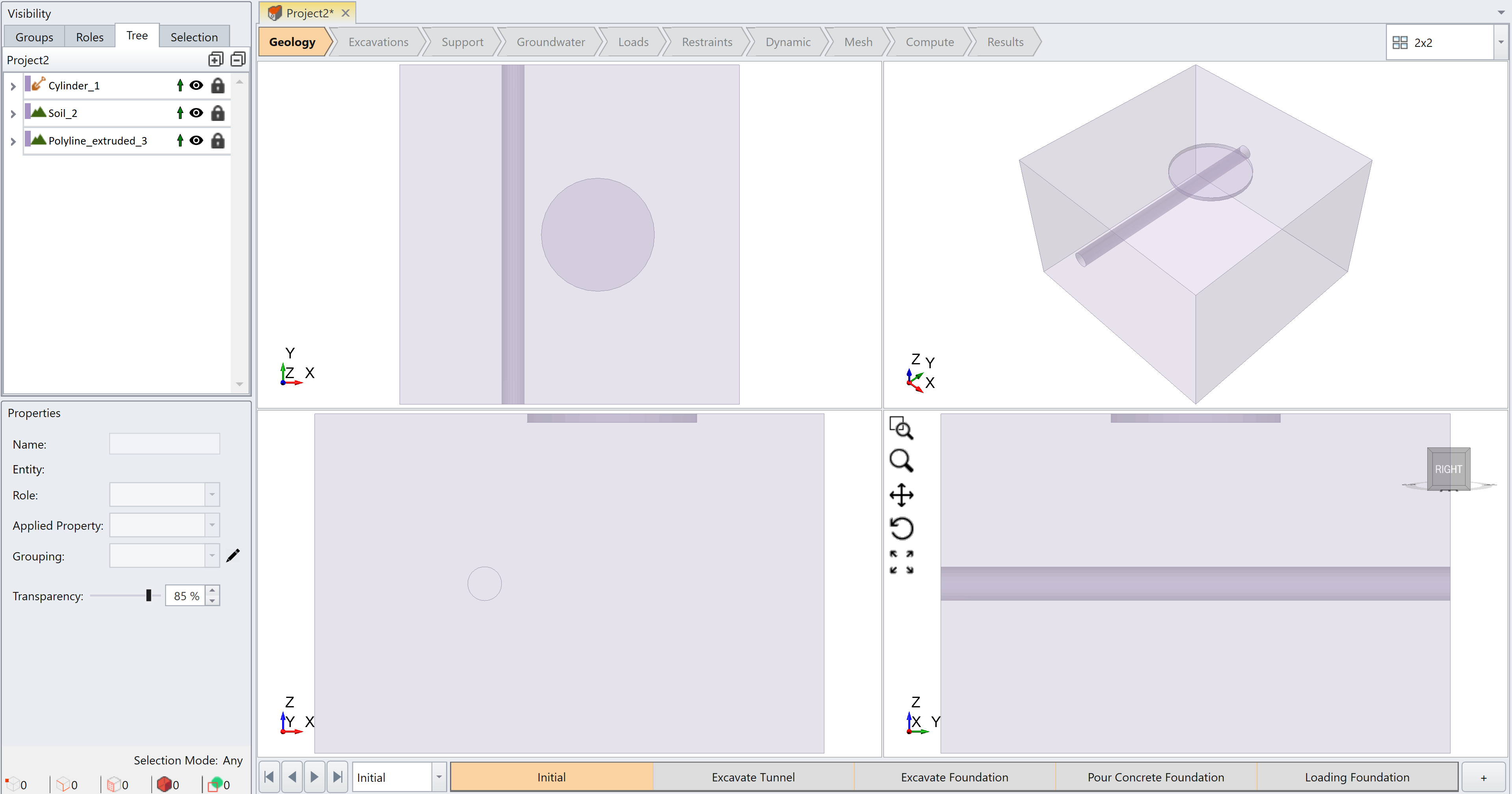
If you look at the visibility pane you will notice that the names of each geometry are labelled with numbers. You can remove the numbers by simply selecting each and changing the names in the properties pane.
- Select each geometry volume in the Visibility pane and name them according to the table below:
Geometry Entity | Name |
Cylinder_1 | Underground Tunnel |
Soil_2 | Soil |
Polyline_extruded_3 | Foundation |
6.0 Staging
6.1 STAGING THE TUNNEL EXCAVATION
The Underground Tunnel is excavated at Stage 2. Therefore in Stage 1 it should still be modeled as “Soil”. While still in the Initial stage, make sure for Underground Tunnel that the Applied Property in the properties pane is set to Soil.
- Now we will move to the Excavate Tunnel stage.
- Select the underground tunnel in the Visibility pane and in the Properties pane change the Applied Property = No Material.
6.2 STAGING THE FOUNDATION
Now we do the same thing for the foundation as we completed for the tunnel, but starting from the Excavate Foundation stage.
- Select the stage tab Excavate foundation.
- Select the foundation volume from the Visibility pane and in the Properties pane, change Applied Property = No Material.
- Now select the Pour Concrete Foundation stage, and in the Properties pane change the Applied Property = Concrete.

7.0 Adding Stress Loading
7.1 APPLYING A SURFACE LOAD TO THE MODEL
- Select the Loads workflow tab

This tab allows you to edit the loading conditions. We will be applying a uniformly distributed load onto the foundation surface.
- Select: Edit > Selection Mode > Faces Selection

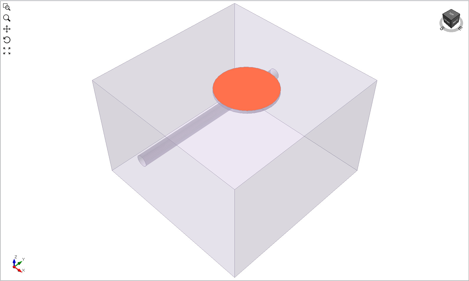
- Select the top face of the foundation either using the XY-plane modeler view or the 3D modeler view. When selected the 3D modeler view should look similar to the following:
- Select: Loading > Add Loads to Selected.
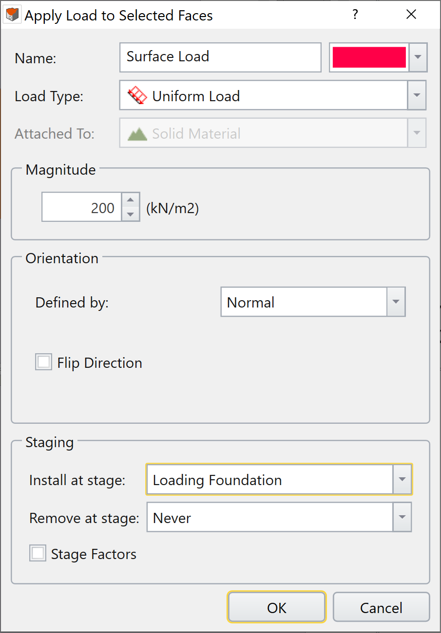
- Enter the following:
- Magnitude = 200 (kN/m2)
- Install at Stage = Loading foundation
- For all other options keep the default values.
- Click OK to save and close the dialog. Before closing you can check to see if your dialog looks like the one below:
7.2 APPLYING A FIELD STRESS
The Field Stress option allows you to edit the field stress loading conditions.
- Select Loading > Field Stress.
- Leave the settings as their default values (e.g. Field Stress Type is set to Gravity).

- Click OK.
8.0 Setting Boundary Conditions
- Move to the Restraints workflow tab
 to assign restraints to the external boundary of the model.
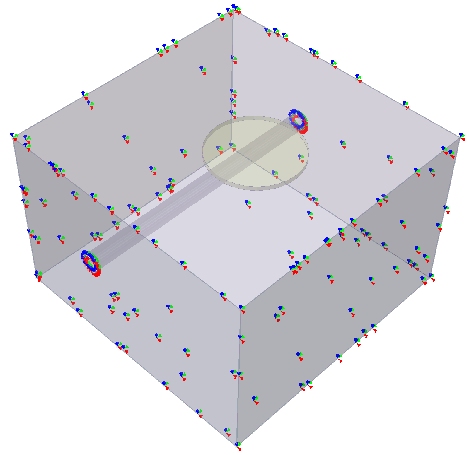
RS3 has a built-in "Auto Restrain" tool for use on underground models. For the purpose of this tutorial we will use the Auto Restrain (Surface) option.
- Select: Restraints > Auto Restrain (Surface)
 . The model should look as the following:
This completes the construction of our model's geometry.
9.0 Meshing
- Next, we move to the Mesh workflow tab

Here we may specify the mesh type and discretization density for our model. For this tutorial, we will use the default settings.
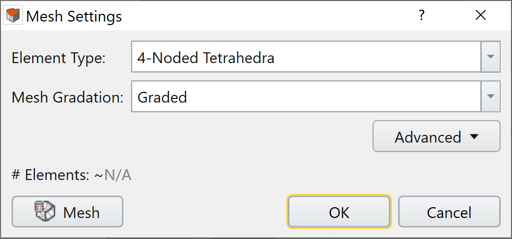
- Select: Mesh > Mesh Settings

- Make sure that Element Type = 4-Noded Tetrahedra and Mesh Gradation = Graded.
- Click Mesh
 to mesh the model. Click OK to close the dialog.
10.0 Computing Results
- Next, we move to the Compute workflow tab

- From this tab, we can compute the results of our model. First, save your model: File > Save As.
- Next, you need to save the compute file: File > Save Compute File.
- You are now ready to compute the results. Select Compute > Compute


11.0 Interpreting Results
11.1 DISPLAYING THE RESULTS
- Next, we move to Results workflow tab

From this tab, we can analyze the results of our model. First, let's refresh the results.
- Select: Interpret > Refresh All Results

On the top right corner of the screen you should see two drop-down menus; Element = Solids and Data Type = Sigma 1 Effective by default.

We will analyze a number of different “Data Type” results. Let’s turn on the exterior contours so we can see some results.
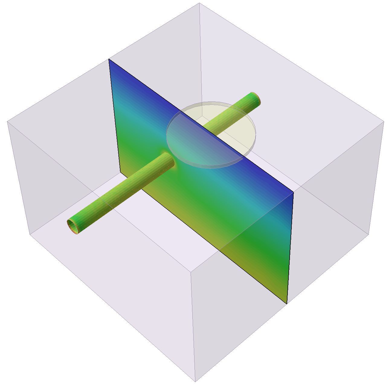
- Select: Interpret > Show Excavation Contour

- Select: Interpret > Show Data on Plane > XZ Plane

- Enter the following origin (x, y, z) = (18, 15, -10).
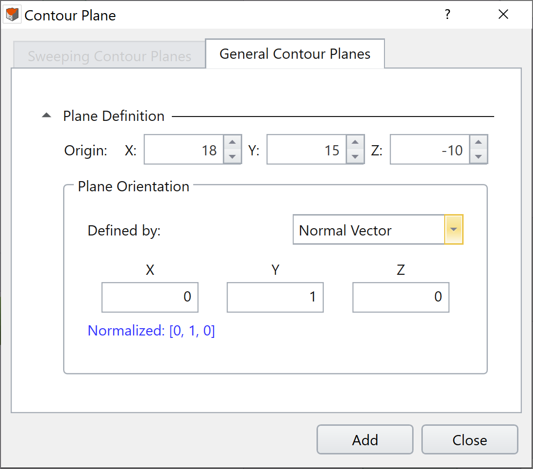
- Select Add and then Close. You should now see a contour plot in the XZ plane.
11.2 DISPLAYING THE PRINCIPAL STRESS RESULTS
In order to compare each stage against each other visually, the contour colour scheme should be standardized across all stages. We can do this by:
- Select: Interpret > Contour Legend > Contour Options

- Select Auto Range (All Stages) as shown below.
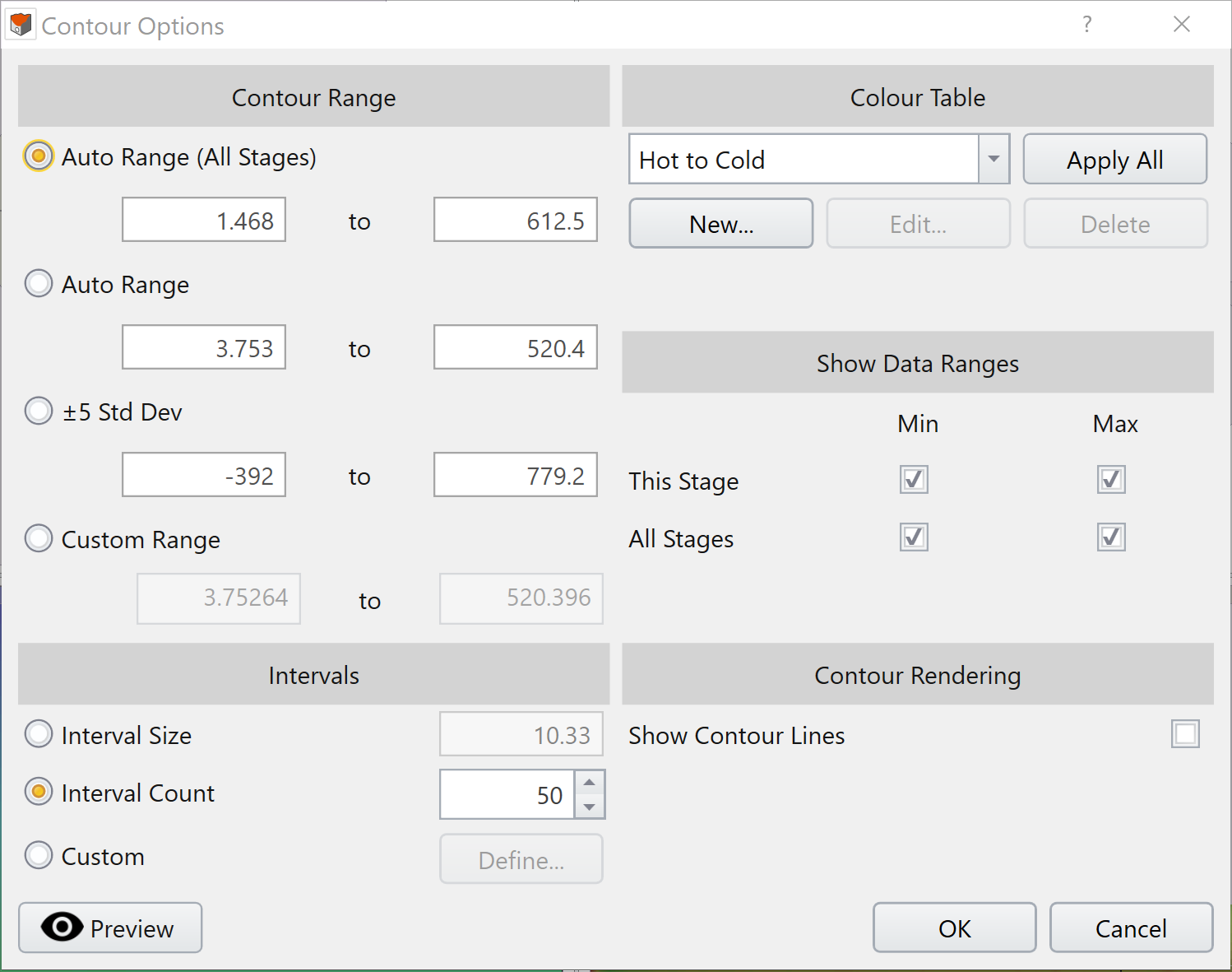
- Click OK
The Sigma 1 Effective results for stages 4 and 5 are shown below in different views:
Sigma 1 effective at Pour concrete foundation (Stage 4) | Sigma 1 effective at Loading foundation (Stage 5) | |
2D view | 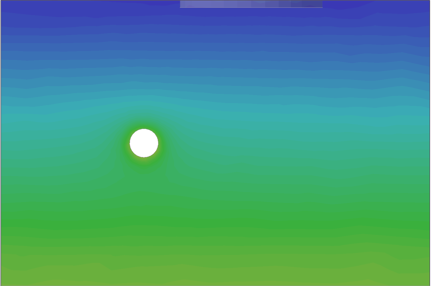 | 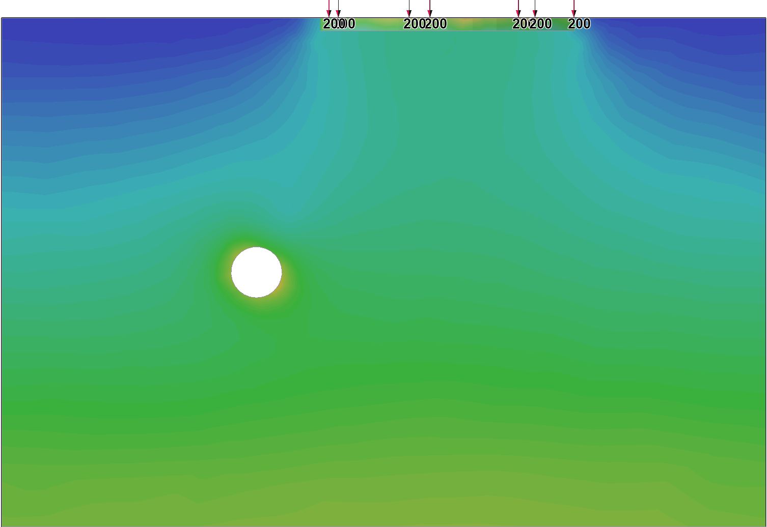 |
3D view | 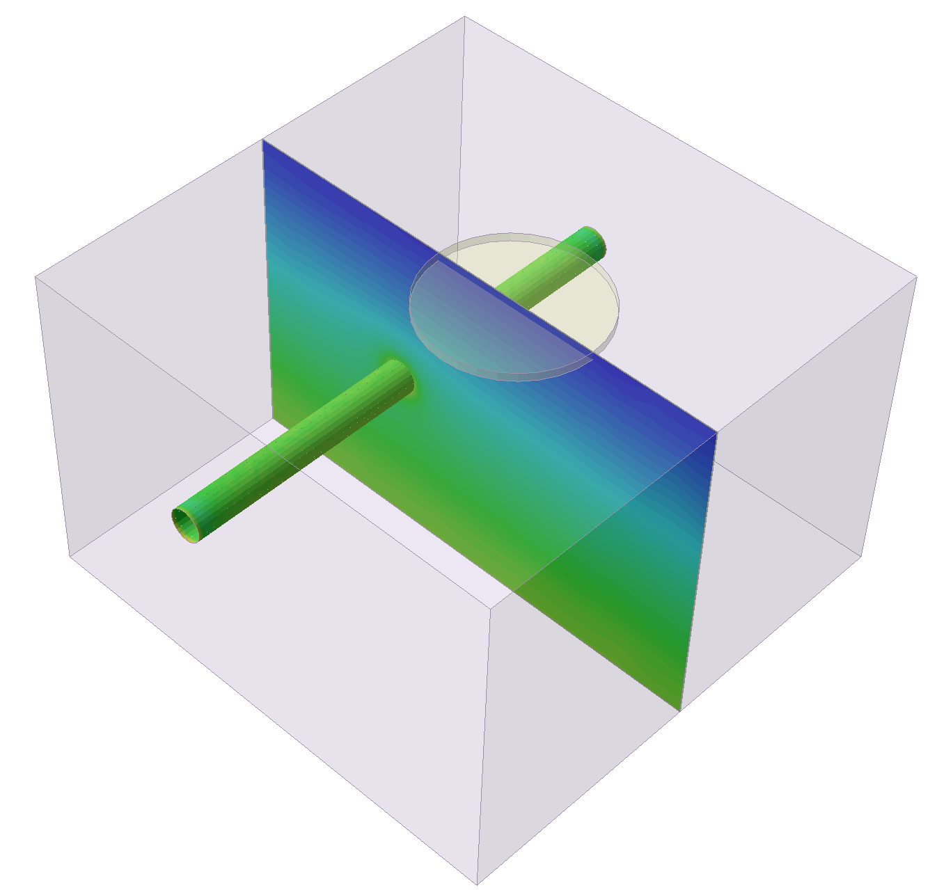 | 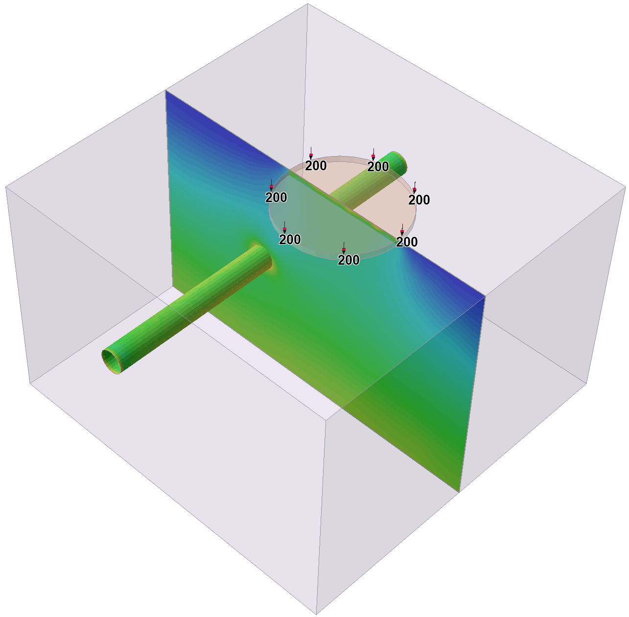 |
Legend |  | 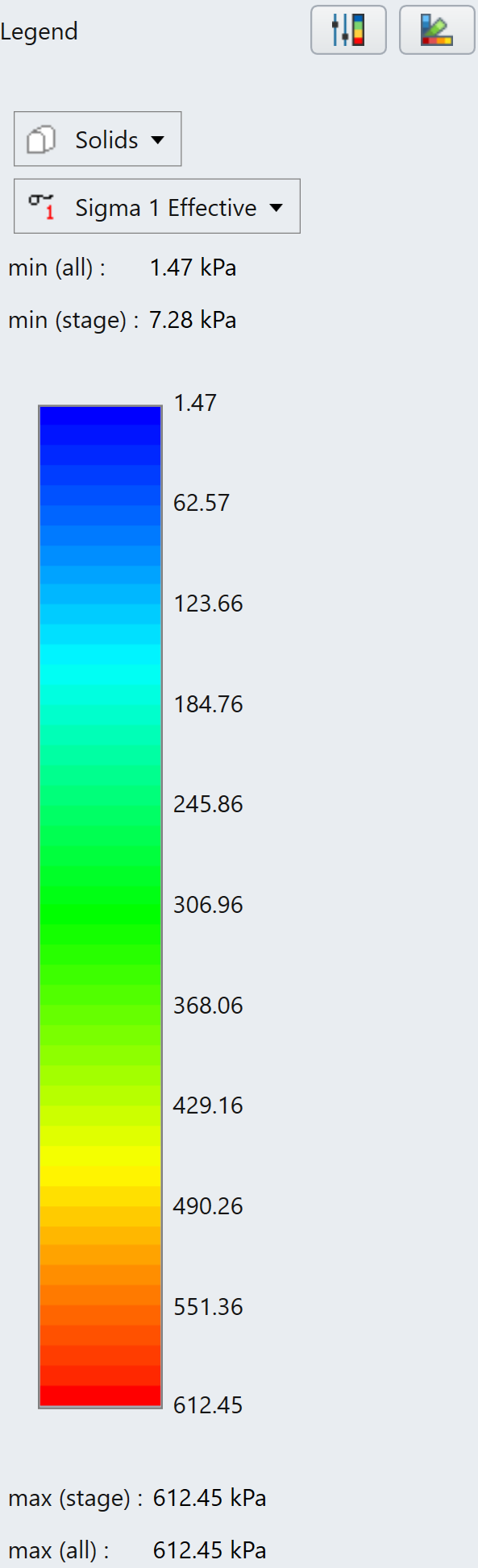 |
As shown in the contour plot, we can see the changes in the stress distribution across the soil model as a load of foundation is applied at stage 5. Next, we will investigate the change in the displacement across stages 2 to 5.
11.3 DISPLAYING THE DISPLACEMENT RESULTS
- In the top right corner of the Results tab, ensure Element = Solids, and change Data Type = Total Displacement

Similar to principal stress result comparison, we will also use auto range across each stage for contour options.
- Select: Interpret > Contour Legend > Contour Options
- Select the check box Auto Range (All Stages).
The Total Displacement results for stages 2 through 5 are shown below in 3D view:
Excavate Tunnel (Stage 2) | 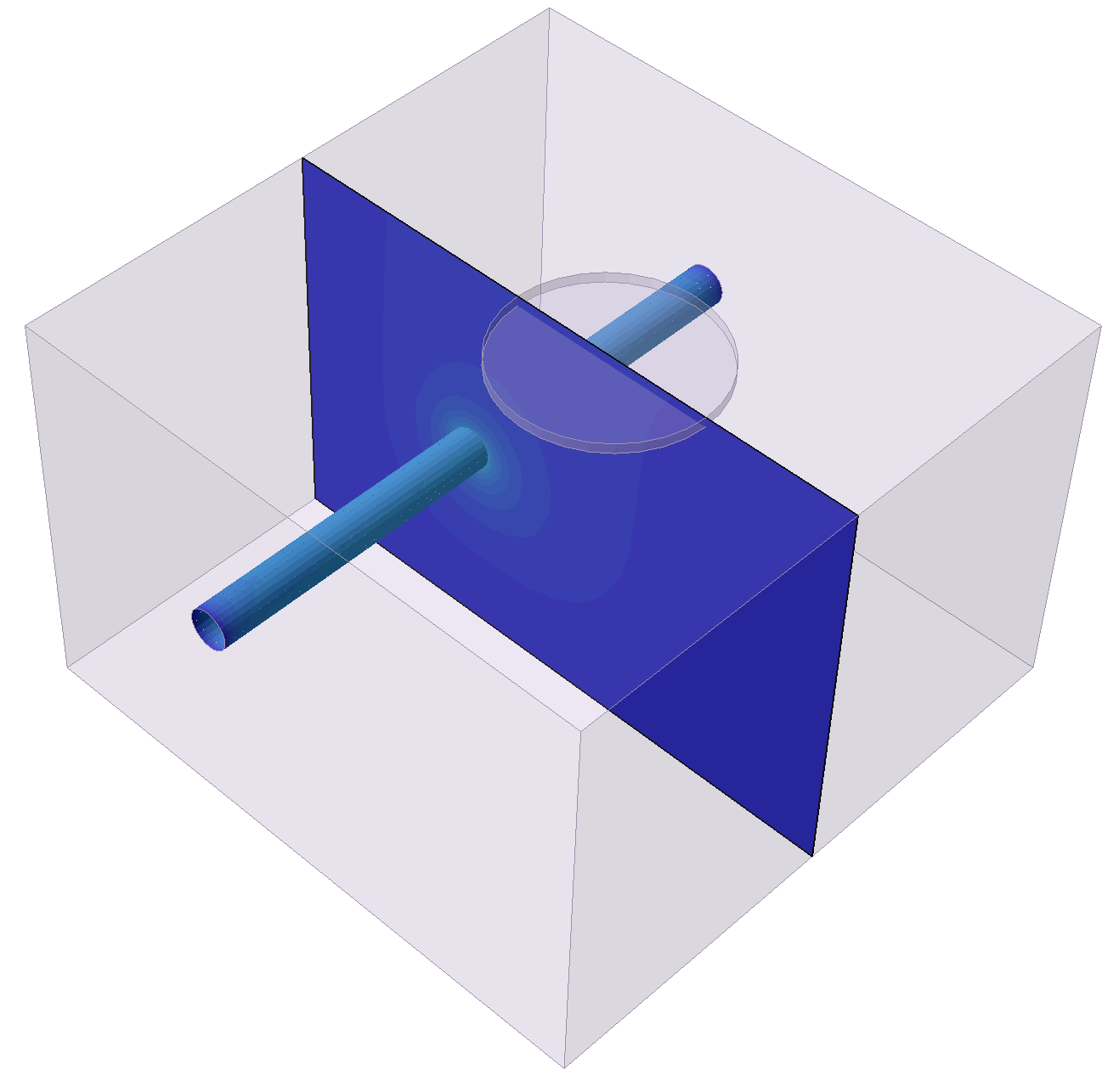 |  |
Excavate Foundation (Stage 3) |  | |
Pour Concrete Foundation (Stage 4) | 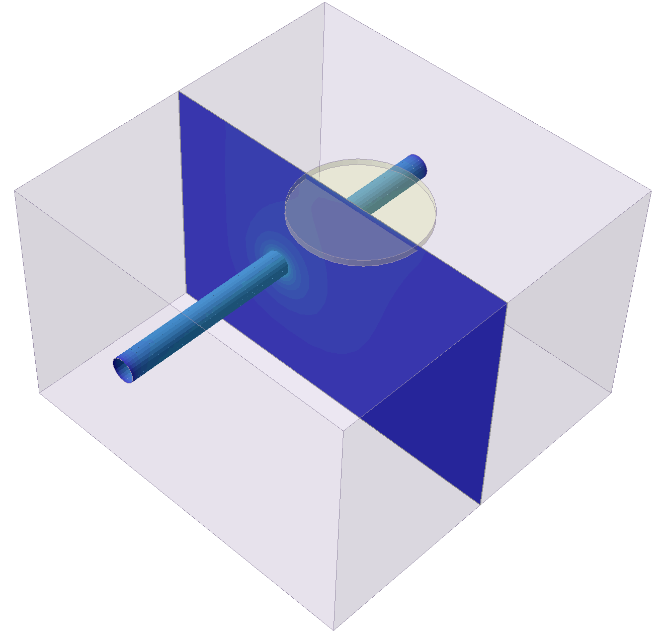 | |
Loading Foundation (Stage 5) | 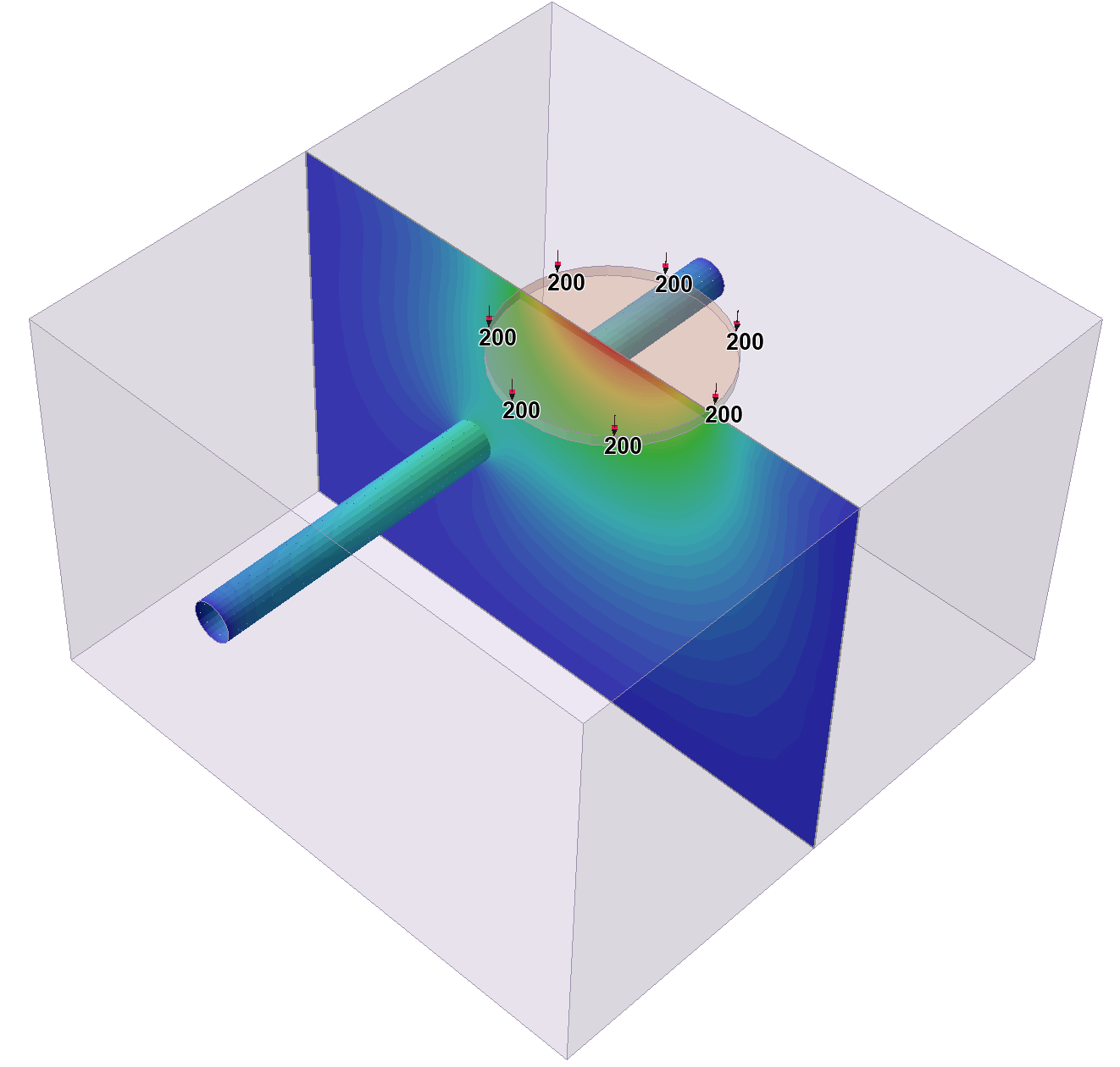 | 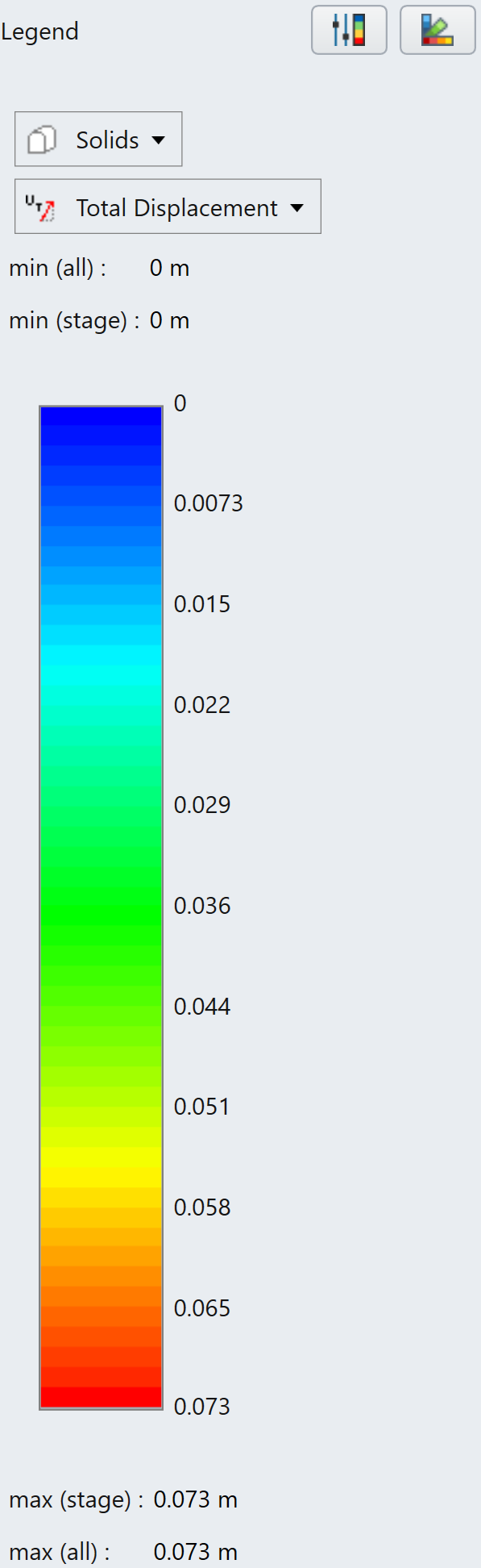 |
This concludes RS3's Quick Start tutorial.