Wick Drains
1.0 Introduction
This tutorial introduces the Wick Drain feature in RS3. Wick drains are installed in soil to improve the rate of seepage when placed to speed up consolidation. In the tutorial, we cover how wick drains are used in the coupled transient analysis model that involves construction of embankment over the stages and also take into account the traffic loading. The modeling results show the effect of wick drains based on the change in pore water pressure and total head distribution.
2.0 Starting the Model
- To start the tutorial, select File > Recent > Tutorials Folder in the main menu.
- Open the starting file Embankment Consolidation-no wick drain.rs3v3.
Because this tutorial focuses on applying wick drains, we will start with a pre-constructed model, which only requires users to add wick drain before computing the model.
- To show all geometry, select View > Show Intersected Geometry.
2.1 PROJECT SETTINGS
We’ll start by checking that the project’s Groundwater and Stages settings are set up appropriately.
- Select Analysis > Project Settings

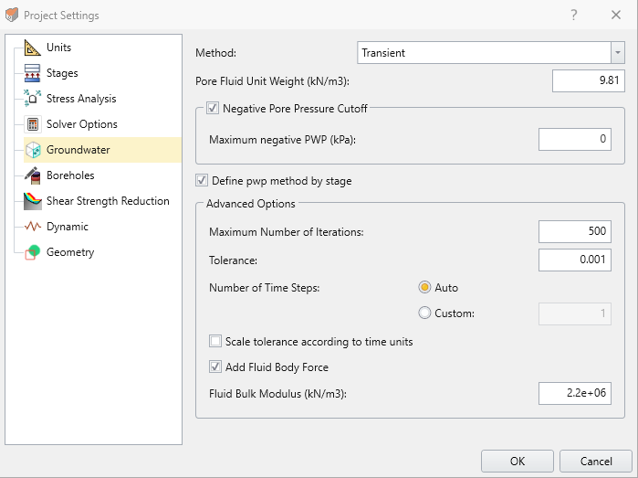
- Select the Groundwater tab to view Method = Transient settings.
- Select the Stages tab to view how the staging is set up.
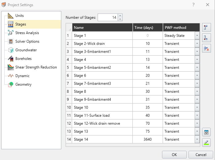
For this tutorial model, the stage setting entries should have already been filled. Note that transient times can be copied and pasted from other file formats, such as .csv, into the Time column.
2.2 MODEL DESCRIPTION
2.2.1 Embankment Construction
The model is designed such that the embankment is constructed by layer over nine stages (Stage 1 - Stage 9). The embankment is divided into four entities that have staged material properties. All four entities have no material property assigned (Applied Property: No Material) at Stage 1. Sequentially, the model is designed in order that the material property named as Embankment Fill is assigned to the embankment entities every other stages from the bottom layer (Stage 3) to the top (Stage 9).
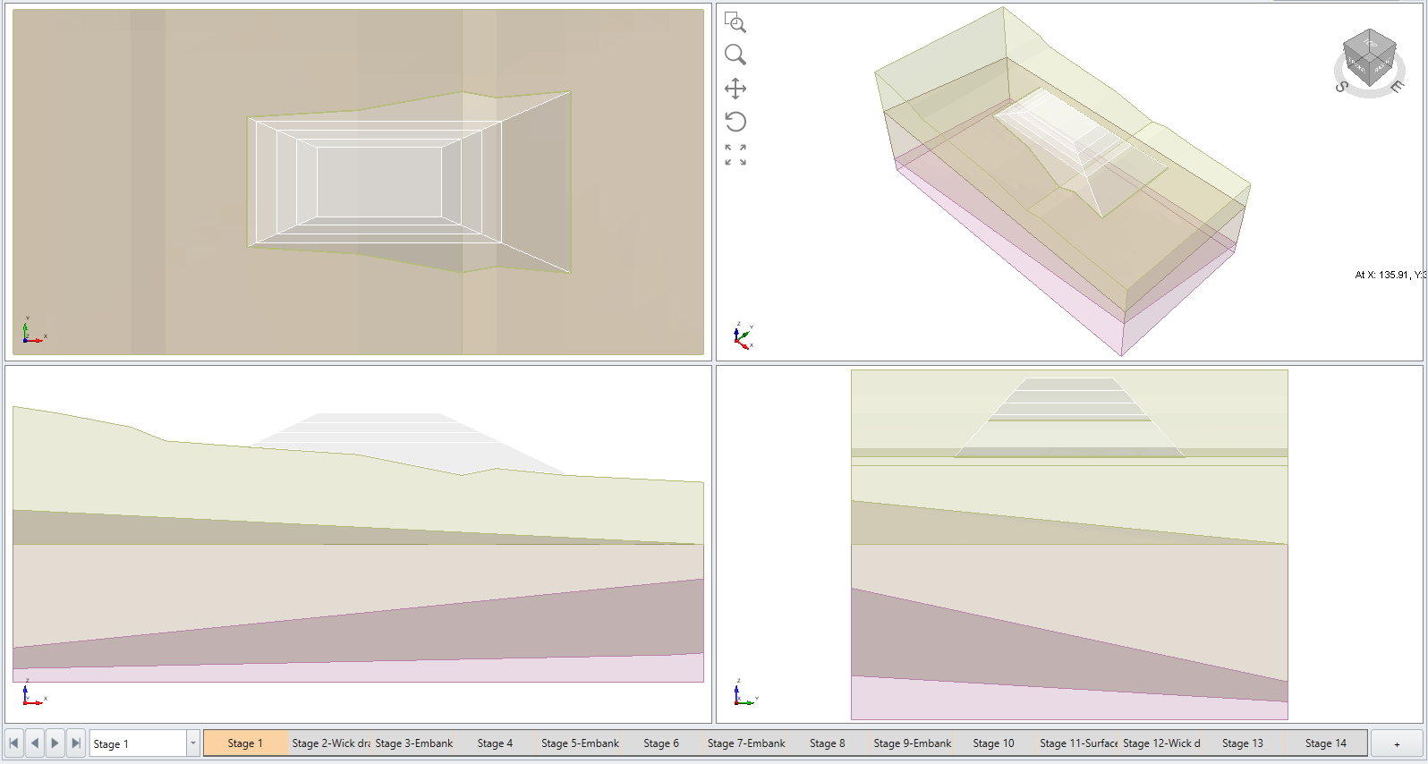
For instance, Stage 1 represents initial condition before embankment construction, as shown below:
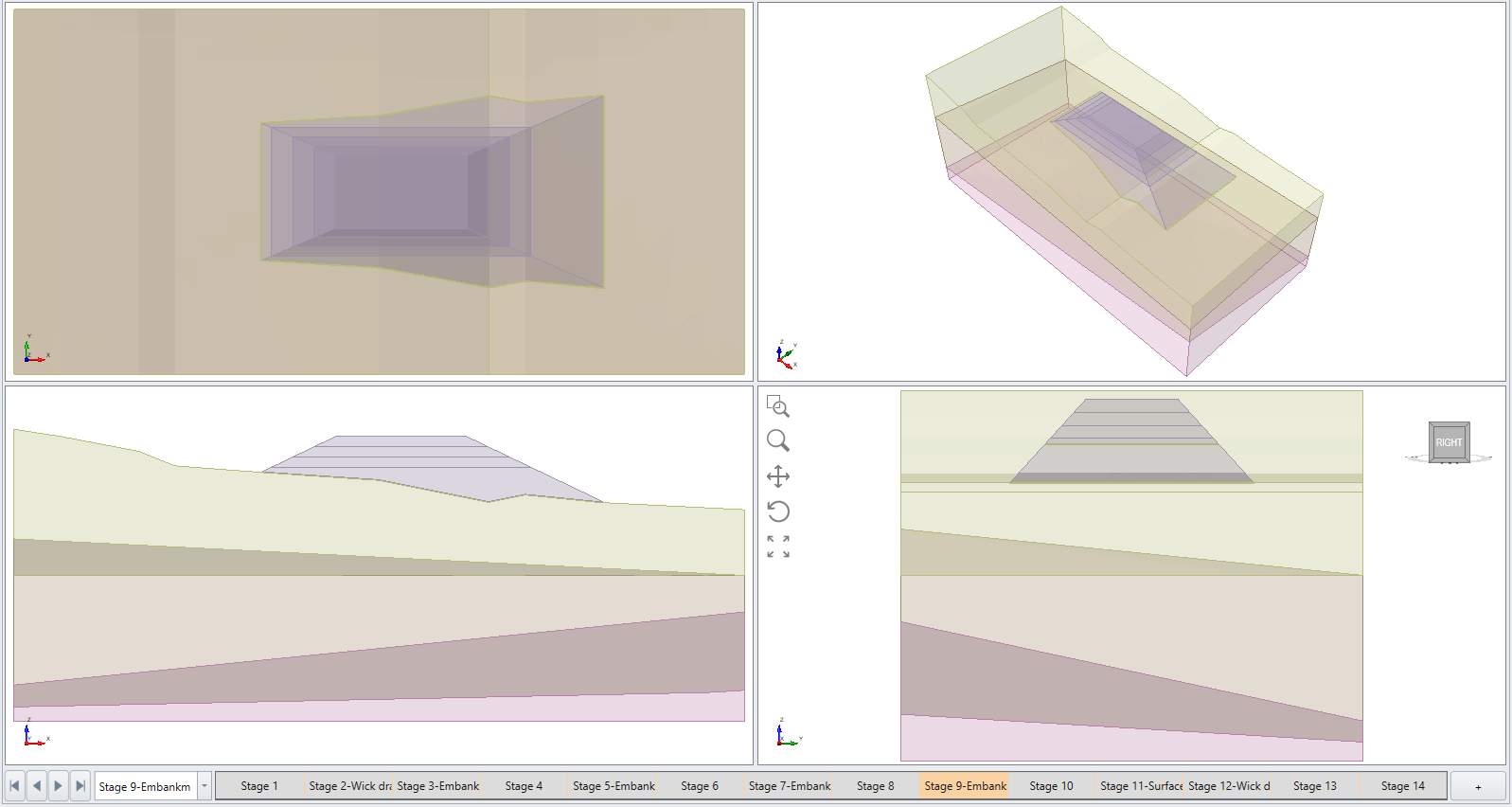
In Stage 9, the model has all embankment entities assigned with Embankment Fill property, representing completed construction of embankment:
2.2.2 Applying Surface Load
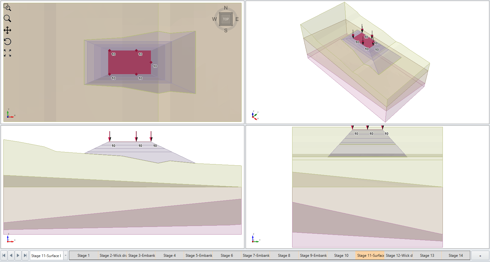
In Stage 11, a surface load of 10 kPa is applied on the top surface of the embankment to represent the load applied by the traffic.
You can check this by switching the workflow tab to the Load workflow tab , wherein the applied surface load will be automatically selected.
2.2.3 Groundwater
- Select the Groundwater workflow tab

This section describes the ground water boundary condition applied to the model. Total Head of -12 m is applied on the left and right face of the soil foundation (represented by Intermediate Layer entities) while an unknown boundary condition is applied on the top surface.
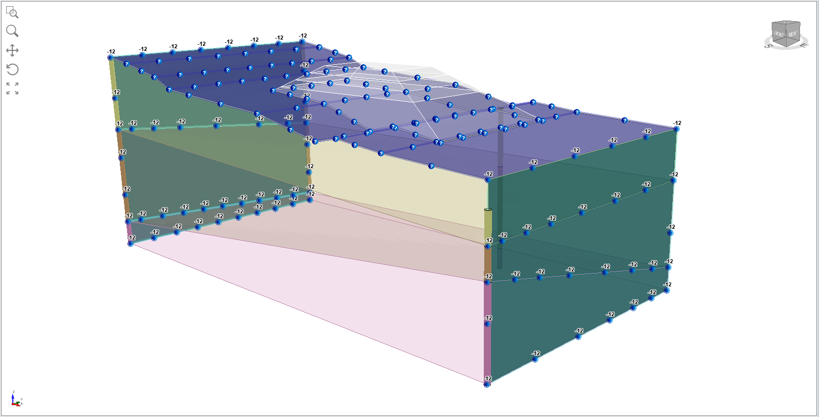
As the embankment is constructed with the stage advancement, the unknown boundary condition is updated accordingly, as such that it is (removed and) re-applied to cover solely the surface of the embankment.

For staged models, like this tutorial model, it often requires an update to the same entities, faces, edges, or vertices for different stages. It may become a cumbersome process to re-select the same item every time a change is made. To overcome such inconvenience, RS3 has a feature to group selected items, in order to avoid the need to reselect them. The Selection Group can be made by
1. Switching to the Selection tab under visibility pane;
2. Selecting any combination of items
3. Clicking the Add a New Selection Group icon under Selection tab.
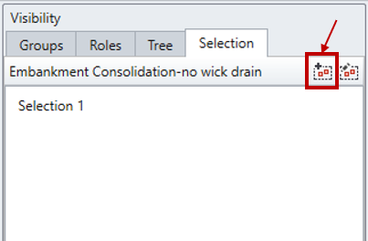
For this tutorial, the Selection group is made for the faces of the top surface of the intermediate layer that is not covered by the embankment to repeat adding the Unknown groundwater boundary condition.
2.2.4 Meshing and Restraints
Additional steps in creating the model include:
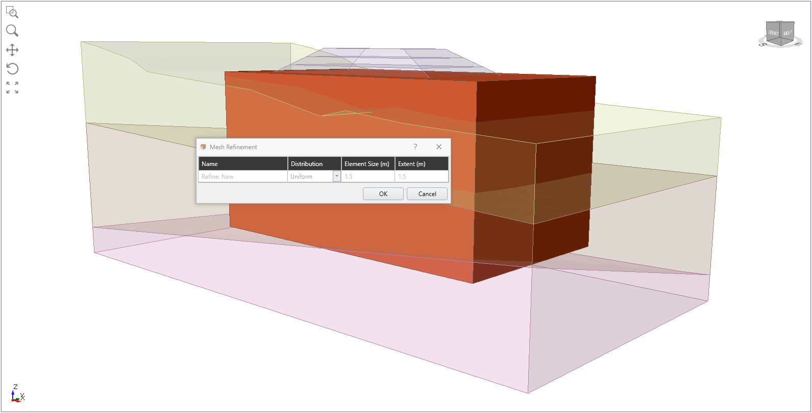
- Defining the mesh refinement region using the box with the uniform element size of 1.5 m.
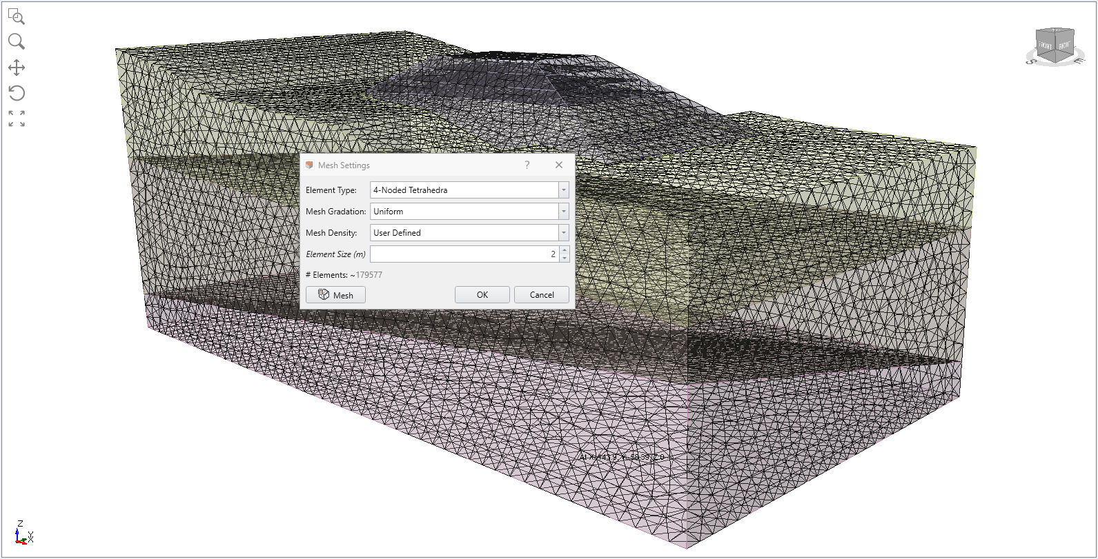
- Meshing the model with uniform element size 2 m.
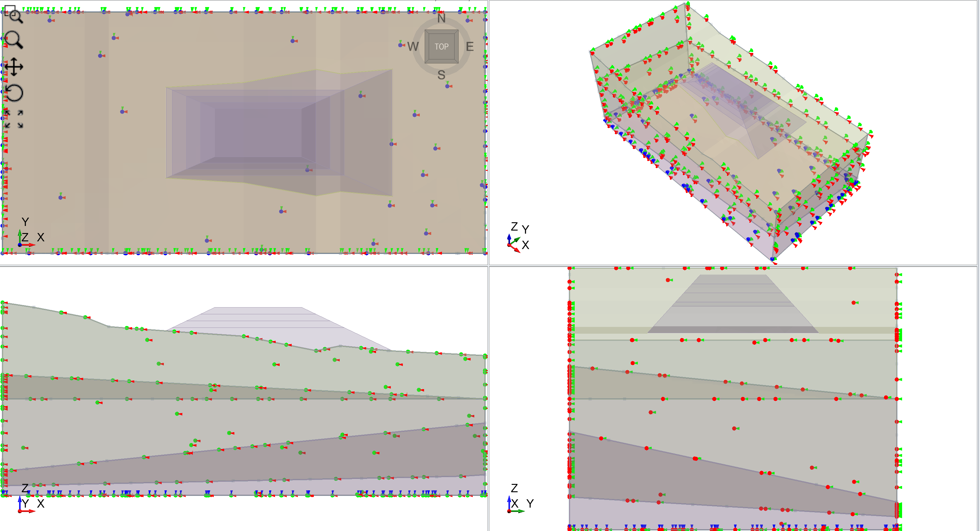
- Applying restraints to fix in x and y direction and all direction on the side surfaces and bottom surface of the foundation, respectively.
3.0 Adding Wick Drains
This section explains the procedure to install wick drains. In this model, wick drains are added in Stage 2.
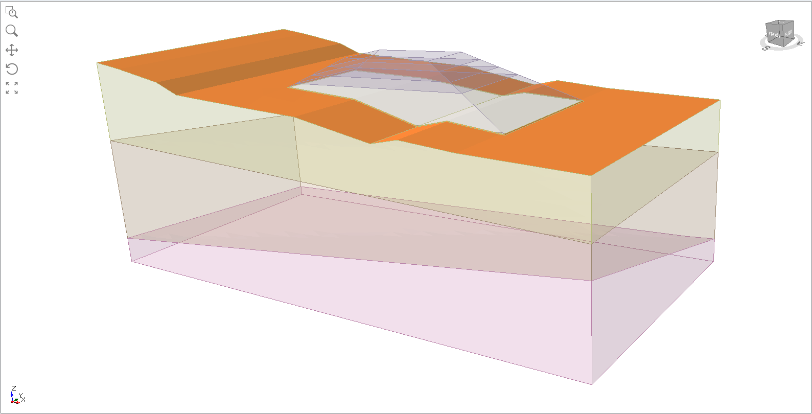
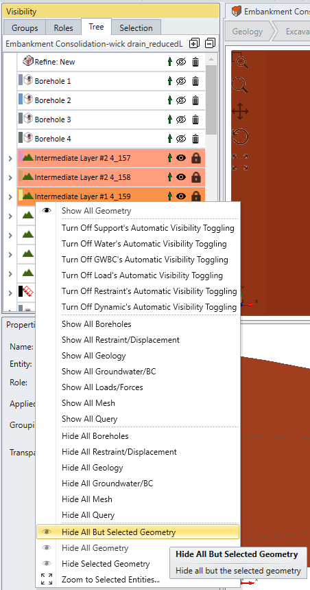
- Select Intermediate Layer entities from the Visibility Tree.
- Right click and select Hide All But Selected Geometry.
- Select: Edit > Selection Mode > Faces Selection
 and select the faces below the embankment.
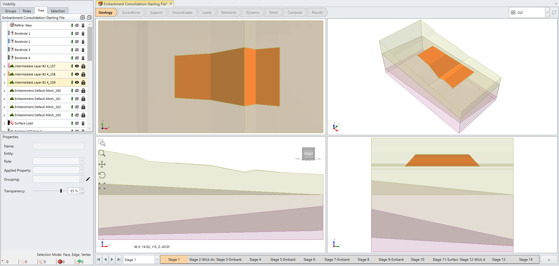 Clicking a part of the surface while holding the shift key selects the whole surface
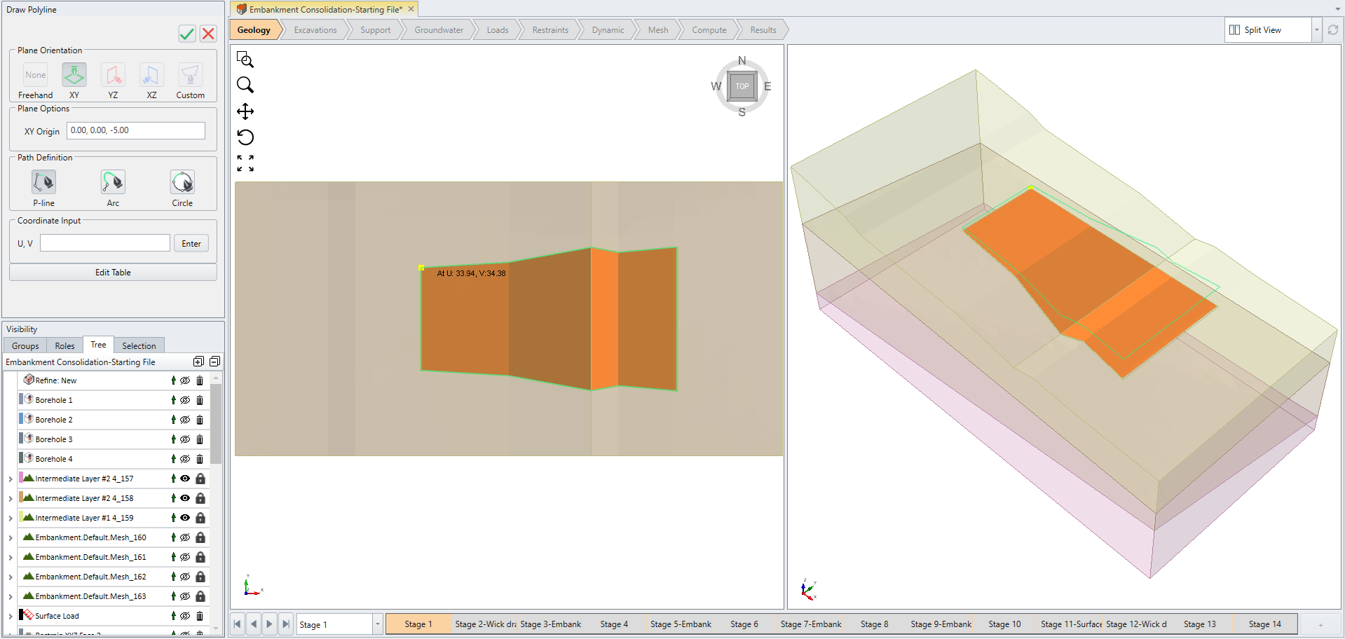
 - Go to Groundwater > Add Wick Drain Region. The Polyline dialog will pop up.
- Under the Plane Options enter XY Orig = (0, 0, -5) and draw a polyline following the edge of selected surface (highlighted in orange)
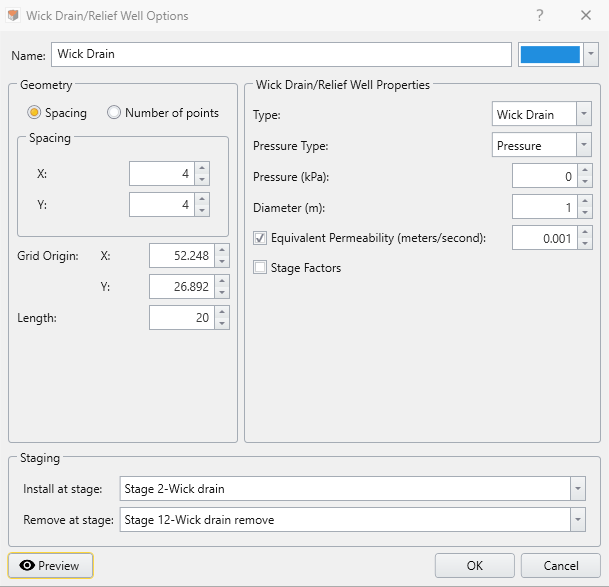
- A Wick Drain/Relief Well Options dialog will appear. Enter the following:
- Spacing: X = 4, Y = 4
- Grid Origin: X = 52.248, Y = 26.892, Length = 20
- Wick Drain/Relief Well Properties:
- Type = Wick Drain
- Pressure Type = Pressure
- Pressure = 0, Diameter = 0.1
- Equivalent Permeability = 0.001
- Install at Stage 2
- Remove at Stage 12
4.0 Compute
- Next, we move to Compute workflow tab

- From this tab, we can compute the results of our model. Before commencing the stress analysis computation, it is recommended to save the final model as a separate file so that you can access the original file anytime: File > Save As.
- Select: Compute > Compute

Stress analysis computation may take some time as this model conducts coupled analysis and non-linear behaviour. Note that the principle of the wick drain is similar to unknown boundary conditions where the pore pressure inside the wick cannot be larger than the input pressure.
5.0 Results
- Next we move to Results workflow tab

The role of wick drain is to increase the rate of seepage to reduce the consolidation time. Therefore, it casts direct impact on pore pressure and vertical displacement is a suitable indicator to monitor the consolidation settlement. The performance of wick drains can be well visualized by placing a contour plane intersecting the wick drains.
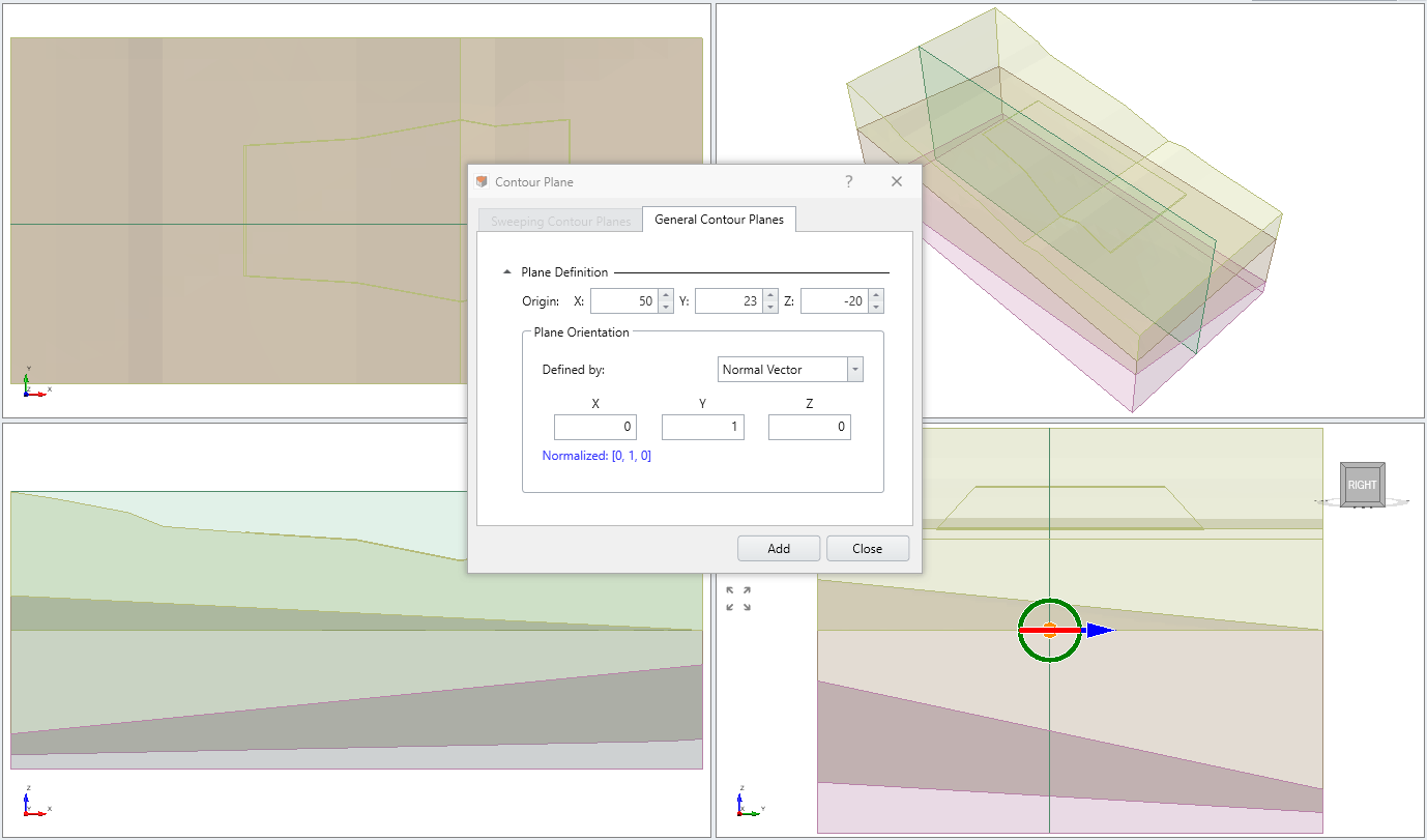
- Select: Interpret > Show data on plane > XZ Plane

- Enter the origin location/orientation of the plane as following:
- X1 = 50, Y1= 23, Z1= -20
- Orientation (X, Y, Z) = 0, 1, 0
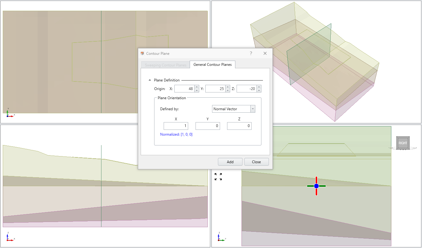
- Add YZ contour plane with following location/orientation:
- X1 = 48, Y1= 25, Z1= -20
- Orientation (X, Y, Z) = 1, 0, 0
5.1 Pore Water Pressure
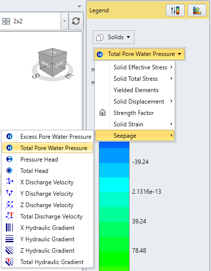
- In the Legend, select the Seepage > Total Pore Water Pressure contour plot.
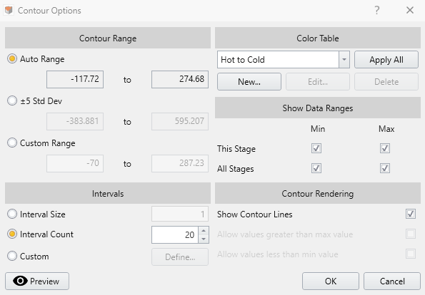
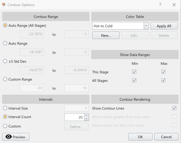
- Click Contour Options
 and Reduce the Interval Count to 20 and with Show Contour Lines enabled.
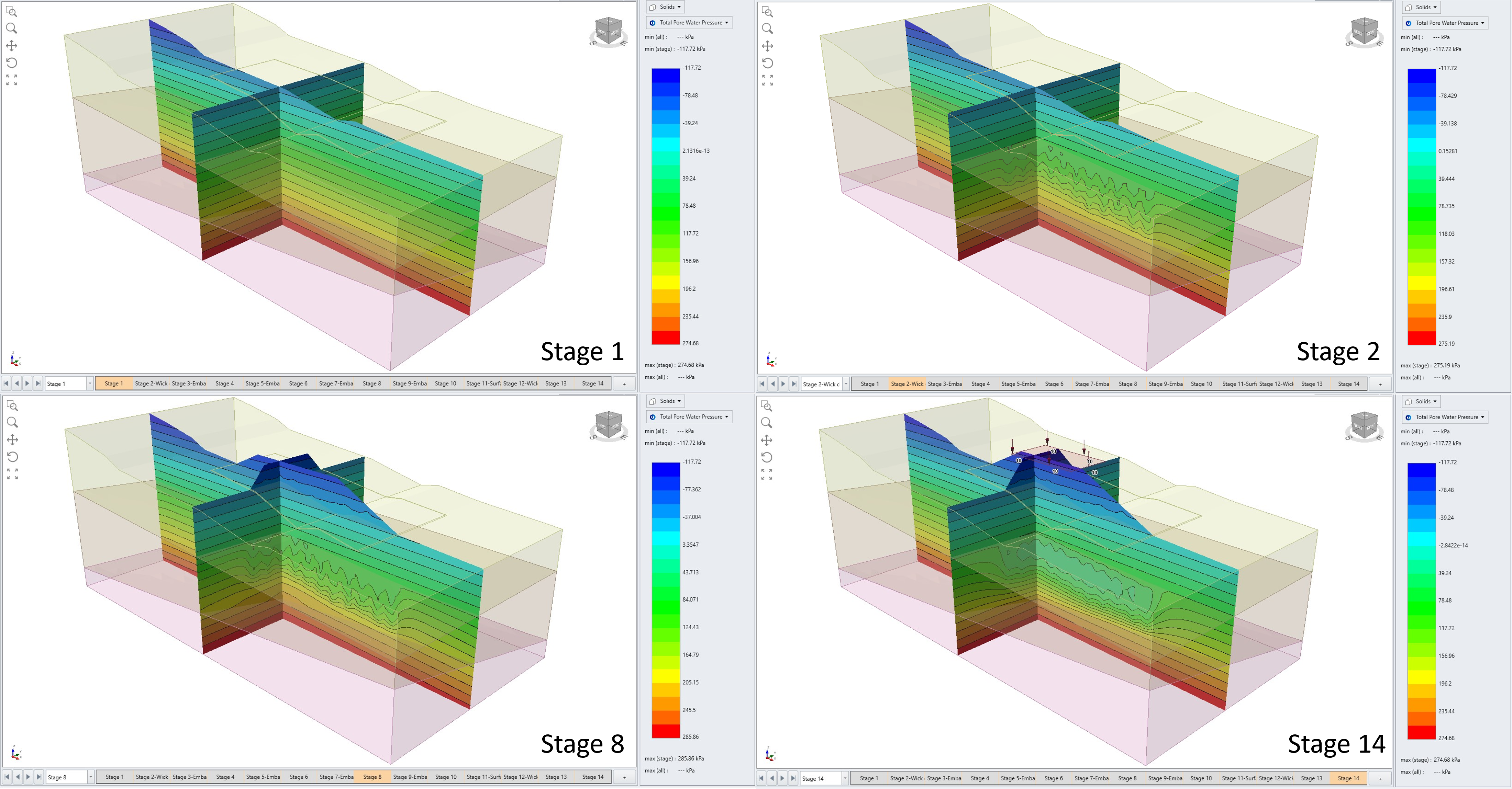
Total pore water pressure distribution for Stage 1, Stage 2, Stage 8, and Stage 14 are presented in the figure below. The modeling results show that along the length of the wick drain, the pore water pressure remains close to or less than 0 kPa.
5.2 Total Head
- In the Legend, select the Total Head contour plot.
- Click Contour Options again. We will keep the same contour options as pore water pressure (20 intervals and showing contour lines). However, for total head, we will use the Contour Range = Auto Range (All Stages) option (which only becomes enabled after loading the total head contour plots for all stages).
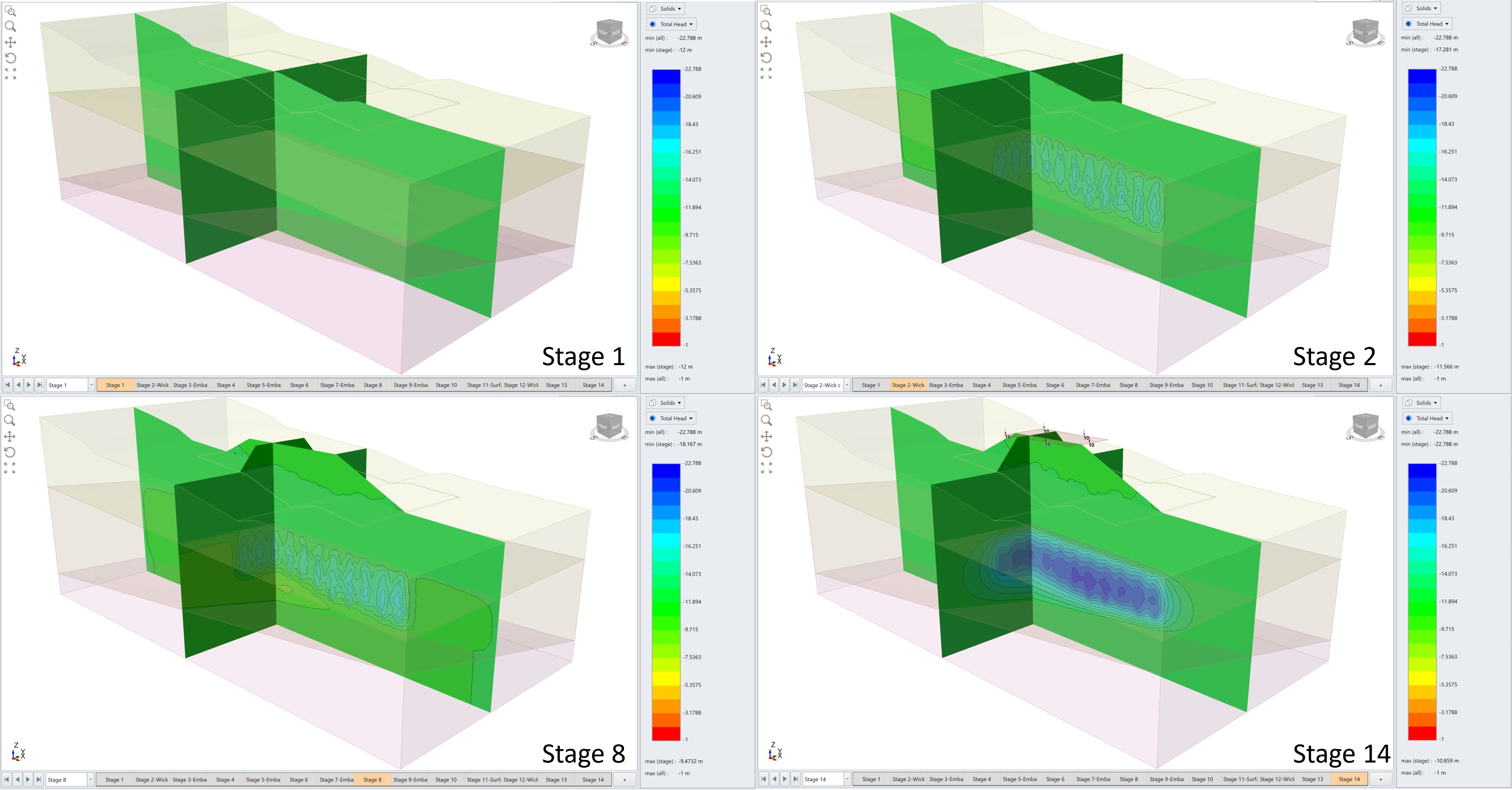
Total head distribution for Stage 1, Stage 2, Stage 8, and Stage 14 are presented in the figure below. The modeling results show a significant reduction in total head around the regions with wick drains installed.
5.3 Z Displacement
- In the Legend, select the Z Displacement contour plot.
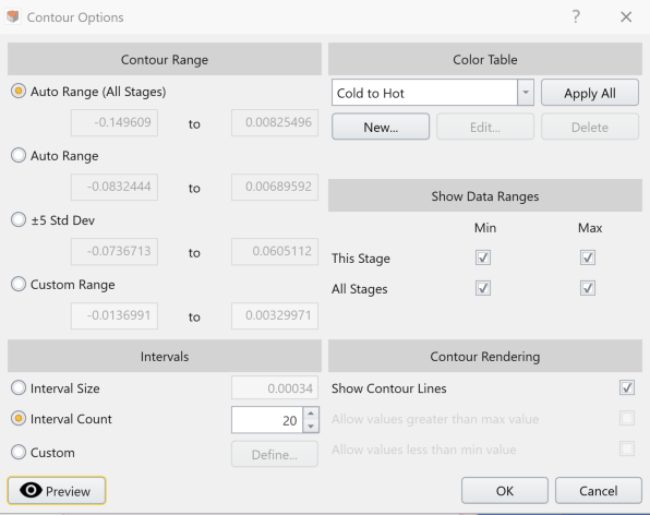
- Adjust the Contour options as following:
- Contour Range = Auto Range (All Stages)
- Interval Count = 20
- Color Table = Cold to Hot
- Show Contour Lines = Enabled
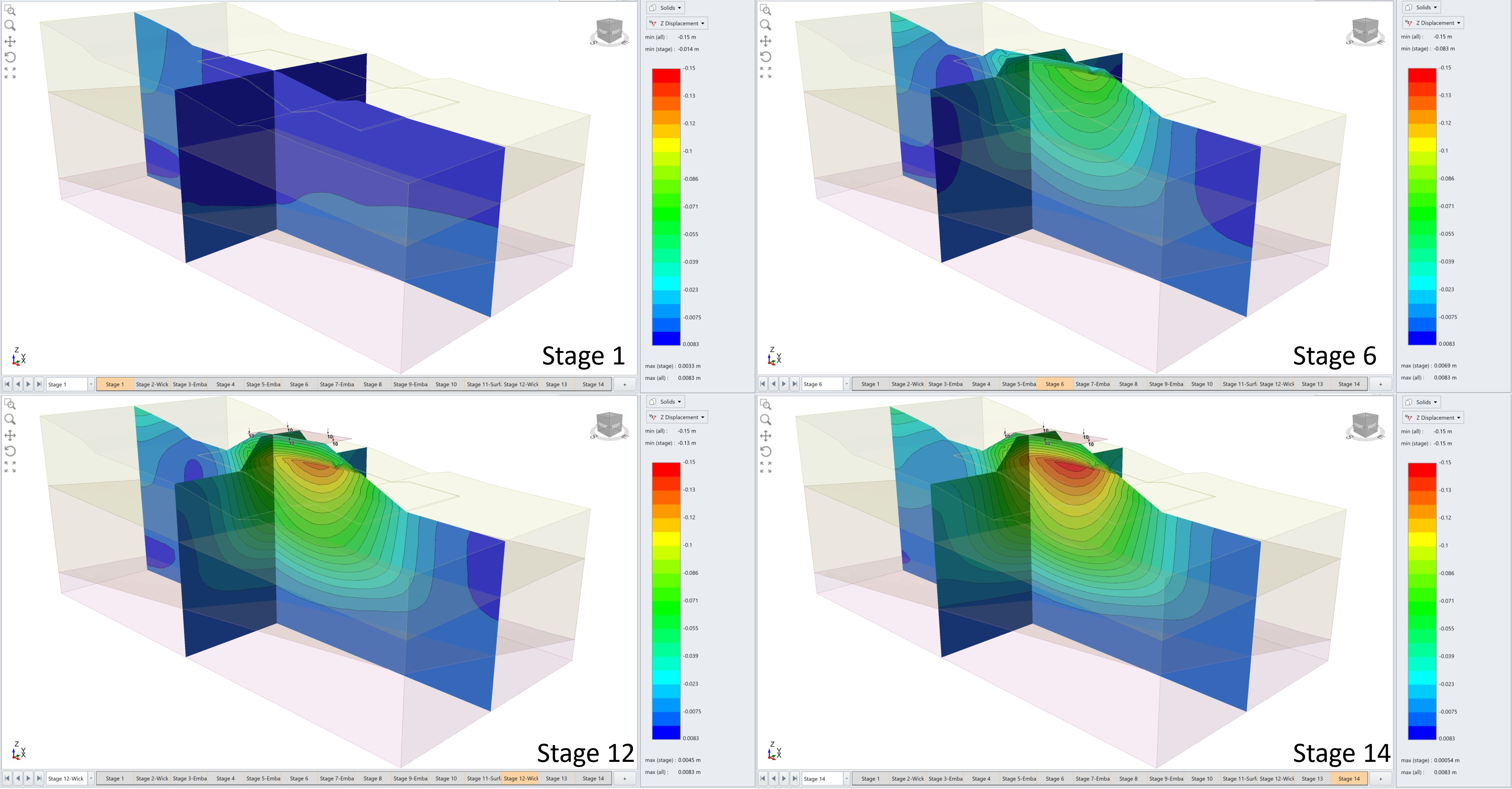
The Z displacement contour plot shows the settlement progression with respect to time.
The magnitude of settlement can be quantitatively compared between stages by using the query point and plotting a z displacement-time graph. To obtain the graph, following steps need to be executed:
- Select: Interpret > Queries > Add Line Query.
- On the Draw Polyline Pane, enter coordinate point 65, 26, -5.2 for X, Y, Z and click Enter.
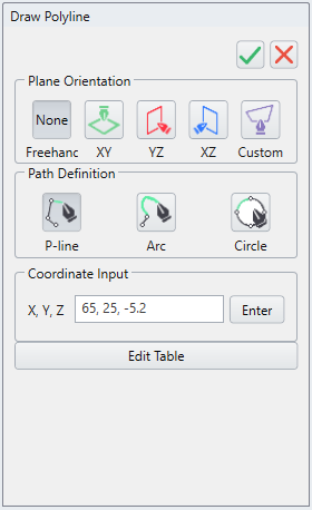
- Click Done

- Select the created Query Line entity from the visibility tree.
- Select Interpret > Graph Data or click the Graph Data
 icon in the toolbar.
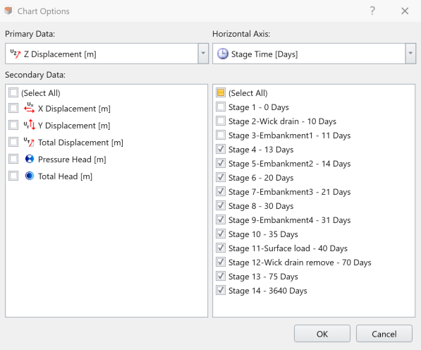
 - Under Chart Options select [Change Plot Data...]
- The Chart Options dialog will appear. Keep the Primary Data = Total Displacement [m], switch Horizontal Axis = Stage Time [Days], and check all stages other than the first three. Click OK.
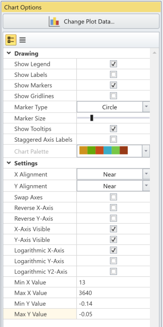
- Under Settings, enable the Logarithmic X-Axis option and enter:
- Min X Value: 13
- Max X Value: 3640
- Min Y Value: -0.14
- Max Y Value: -0.05
Following the above mentioned procedures, the Stage Time [Days] - Z Displacement [m] graph should be generated as below:
![Stage Time [Days] - Z Displacement [m] graph](https://static.rocscience.cloud/assets/help/rs3/tutorials/05-wick-drains/Time-disp-graph.png)