Axisymmetric Analysis
1.0 Introduction
This tutorial will illustrate the axisymmetric modelling option in RS2. Axisymmetric modeling allows the user to analyze a 3-D excavation which is rotationally symmetric about an axis. The input is 2-dimensional, but the analysis results apply to the 3-dimensional problem.
An axisymmetric model in RS2 is typically used to analyze the end of a circular (or nearly circular) tunnel. The model analyzed in this tutorial represents the end of a cylindrical tunnel of 4-meter radius.
Note:
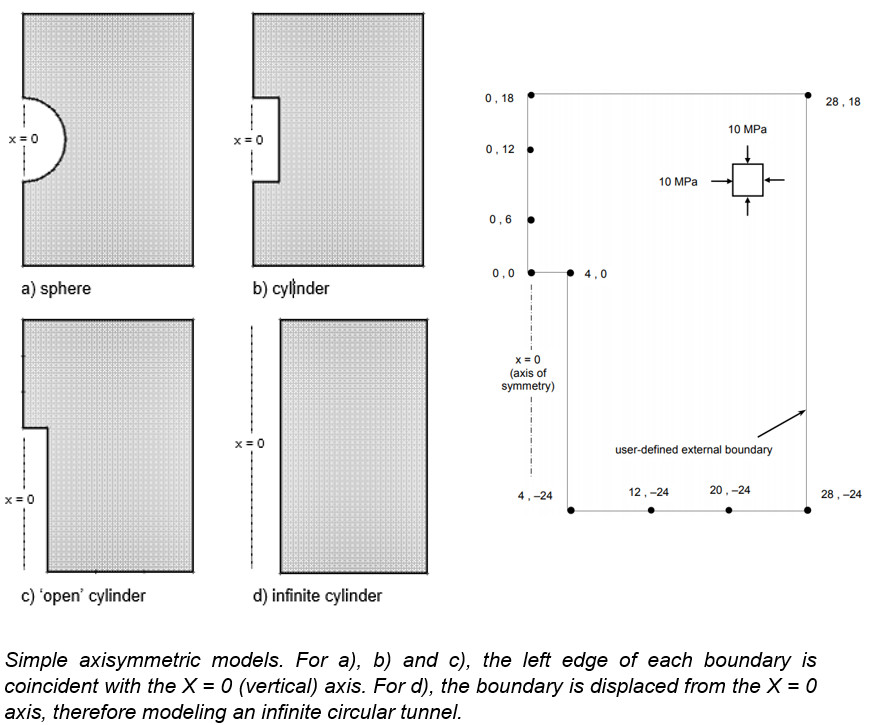
- Only an external boundary is necessary to define an axisymmetric model – the excavation is implicitly defined by the shape and location (relative to the x=0 axis) of the external boundary. Appropriate boundary conditions must also be applied to complete the modelling.
- The axis of rotation is always the X = 0 (vertical) axis. The model must always be mapped to fit this convention, regardless of the actual orientation of the excavation. Because of the symmetry, only “half” of the problem needs to be defined.
To visualize an axisymmetric excavation, imagine the shape formed by rotating the external boundary about the x=0 axis. Note that the previous figure is for illustration and that the boundaries should be extended relative to the excavations (in Figures a. and b., to ensure that the fixed boundary conditions do not affect the results around the excavation). Figure d. can be defined by a narrow horizontal strip since the problem is effectively one-dimensional (i.e. results will only vary along a line perpendicular to the tunnel) and is equivalent to a circular excavation in a plane strain analysis.
There are various restrictions on the use of axisymmetric modelling in RS2, for example:
- The field stress must be axisymmetric i.e., aligned in the axial and radial directions.
- Cannot be used with BOLTS (however LINERS are permitted).
- All materials must have ISOTROPIC elastic properties.
This tutorial examines results around the end of the tunnel as well as along its length, where the conditions are effectively plane strain. Later, the results will be verified by comparing with a plane strain analysis.
2.0 Compute
- Select: File > Recent Folders > Tutorial Folder and open Axisymmetry Tutorial Part 1
- Select: Analysis > Compute

3.0 Results and Discussion
- Select: Analysis > Interpret

3.1 Sigma 1
On the Sigma 1 contours, notice the stress concentration at the ‘corner’ of the tunnel (remember the tunnel is circular).
- Toggle the Stress Trajectories
 on.
on.
The principal stress trajectories illustrate the “stress flow” around the end of the tunnel.
The square dot markers in the upper right corner of the model indicate nodes where the difference between Sigma 1 and Sigma 3 is less than a certain tolerance, so that the conditions are effectively hydrostatic, and a distinction between ‘major’ and ‘minor’ principal stress is not warranted.
- Toggle the stress trajectories off by re-selecting the Stress Trajectories toolbar button.
Look at Sigma 3 and Sigma Z and consider the significance of the principal stress results from an axisymmetric analysis. As with plane strain, Sigma 1 and Sigma 3 are the major and minor ‘in-plane’ principal stresses. Sigma Z is therefore the ‘out-of-plane’ stress, however, since the problem is axisymmetric, Sigma Z is really the induced circumferential or hoop stress around the excavation.
3.2 Displacement
- Now let’s view the displacements by selecting Total Displacement from the drop-down menu in the toolbar.
- Now let’s view the deformation vectors. Right-click and select Display Options.
- Toggle Deformation Vectors on and enter a scale factor of 600.
- Select Done.
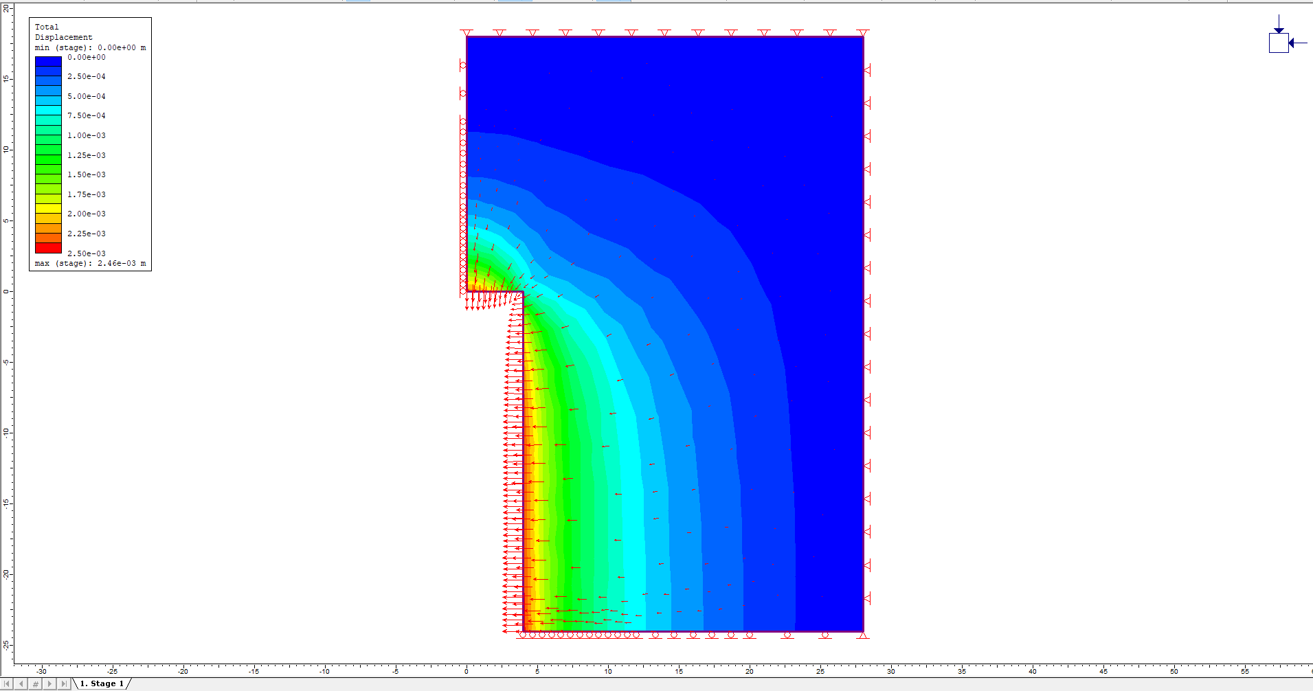
The deformation vectors show the inward displacement along the length and face of the tunnel. Notice how the “corner” of the tunnel effectively restrains the displacements in both x and y directions.
- Toggle the deformation vectors off by selecting the Deformation Vectors button in the toolbar.
3.3 Query Data
RS2 allows users to query data anywhere in the rock mass to obtain values interpolated from the contour plots. A query can be a single point, a line segment, or an arbitrary polyline.
Let’s first create a query along the length of the tunnel.
- Select: Query > Add Material Query

- It will be handy to use the Snap option, so right-click the mouse and make sure the Snap option is selected. While in Snap mode, placing the cursor near a vertex will snap exactly to the location of that vertex.
- Use the mouse to select the vertex at (4, 0).
- Use the mouse to select the vertex at (4, -24).
- Right-click the mouse and select Done. The following dialog will appear:
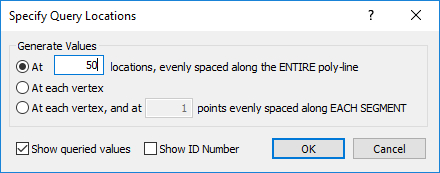
- In the Specify Query Locations dialog, select the first option for Generate Values, and enter a value of "At 50 locations, evenly spaced along the ENTIRE poly-line." Uncheck the option for Show ID Number. Click OK.
Along (4,0) and (4,-24), 50 evenly spaced material queries are created with shown values.
3.4 Graphing a Query
Graphs are created from queries with the Graph Material Queries option. However, a convenient shortcut to graph data for a single query, is to simply right-click on a query and select Graph Data.
- Right-click on the query (i.e. anywhere along the length of the tunnel) and select Graph Data from the popup menu.
- In the Graph Query Data dialog, select Plot to graph the total displacement along the length of the tunnel. Because the Total Displacement contours were turned on, graphing the query displayed a graph of total displacement vs. distance along the query. The data graphed always corresponds to the contoured data being viewed.
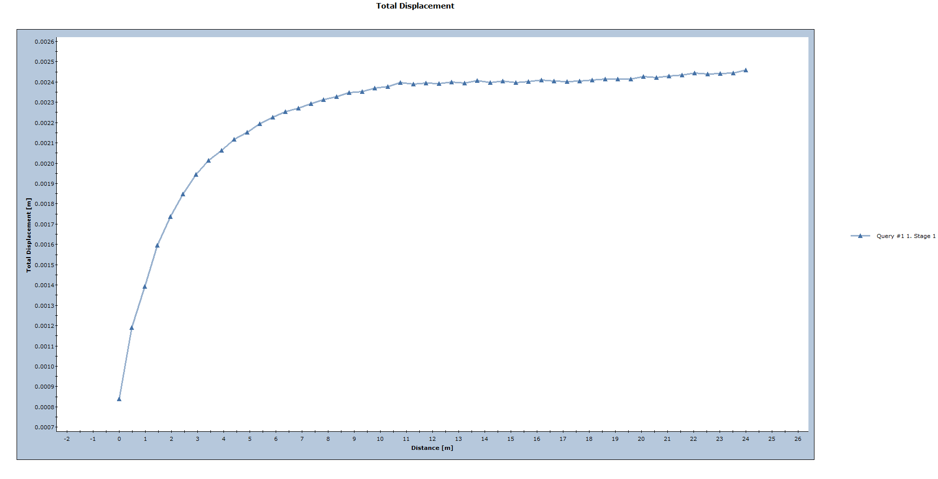
The displacement levels off and becomes constant at a certain distance away from the tunnel face. This curve is useful because it shows the distance at which end effects can be ignored and plane strain conditions can be assumed. This curve can also be used to estimate the “load split” factors, as described in the Support Tutorial.
3.5 Deleting a Query
Now let’s create two more queries, this time perpendicular to the tunnel, and plot them on the same graph.
- Select: Query > Add Material Query
- The Snap option should still be in effect, so use the mouse to select the vertex at (4, -24), and then select the vertex at (28, -24). Right-click the mouse and select Done.
- In the Specify Query Locations dialog, enter 50 locations and select OK.
- Add another query by selecting Query > Add Material Query

- Use the mouse to select the vertex at (4, 0).
- Now enter the coordinates (28, 0) in the prompt line. Alternatively, right-click and select the Ortho snap option, which will allow the user to snap the query exactly along a horizontal line and to the external boundary (at the point 28,0) because the Snap option is also enabled. Right-click the mouse and select Done.
- In the Specify Query Locations dialog, enter 50 locations and select OK.
Two new queries have been created, one along the lower edge of the model, and a parallel one at the face of the tunnel.
To graph both queries on the same plot, use the Graph Material Queries option (the right-click shortcut can only be used to graph a single query).
- Select: Graph > Graph Material Queries
- Select the two queries by clicking on them.
- Right-click and select Graph Selected (or press Enter)
- In the Graph Query Data dialog, click Plot to obtain the following graph:
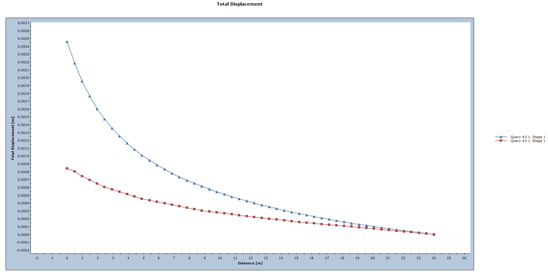
The total displacement decreases further from the tunnel.
Note:
- The Total Displacement along the lower boundary is exactly equivalent to the Horizontal (X) Displacement, since the Vertical (Y) Displacement along this boundary is zero.
- The Total Displacement curve at the face of the tunnel includes both X and Y displacement components.
Now close the graph view by selecting the X in the upper right corner of the view (or right-click and select Close Chart).
3.6 Plane Strain Comparison with Axisymmetric Results
To further illustrate the significance and meaning of an axisymmetric model, let’s look at a plane strain model which is equivalent in all respects to the axisymmetric model (except that the tunnel will now be infinite, with no ‘end effects’), and compare the analysis results.
- Select: File > Recent Folders > Tutorial Folder and open Axisymmetric Tutorial Part 2.fez.
- Select: Analysis > Compute
- Select: Analysis > Interpret
- View the total displacement contours by selecting Total Displacement from the drop-down menu in the toolbar
Notice the maximum displacement displayed in the status bar (0.00245m).
This is almost identical to the maximum displacement from the axisymmetric problem (0.00246m).
Now let’s use the Query and Graph options again to plot the displacement vs. distance from the tunnel boundary.
- Select: Query > Add Material Query
- Enter the point (4, 0) at the first prompt and (28, 0) at the second prompt. Right-click and select Done, or press Enter.
- In the Specify Query Locations dialog, enter 50 locations and select OK.
- Notice the query created from the right edge of the tunnel to the right edge of the external boundary. Right-click on the query and select Graph Data.
- In the Graph Query Data dialog, click Plot. A graph of total displacement will be generated.
The displacement is decreasing from the maximum at the tunnel boundary to zero at the fixed external boundary.
Finally, let’s compare this curve with the equivalent query from the axisymmetric analysis.
- Open the axisymmetric model (axi1.fez) in the Interpret program.
- Right-click on the lower query (at the bottom edge of the model) and select Graph Data to generate the graph.
- Now tile the views by selecting Tile Windows from the toolbar to obtain the following:
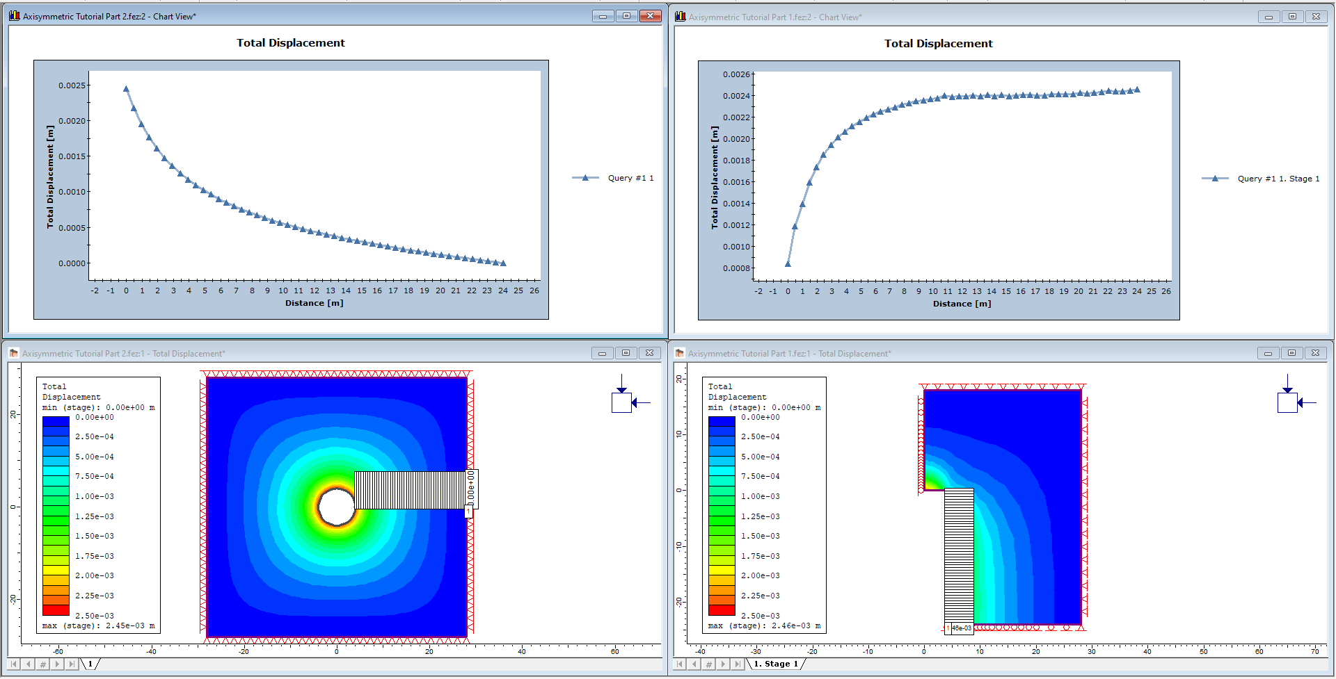
The Total Displacement graphs from the two models are nearly identical.
- One graph represents the query along the lower edge of the axisymmetric model.
- The other is the query added on the plane strain model.
This illustrates the relationship between the axisymmetric and plane strain models; although the two models look very different, the same results can be extracted from either one.
4.0 Additional Exercises
When the total displacement contours were plotted for the plane strain tunnel model, the contours begin to get “square” with increasing distance from the tunnel (immediately around the tunnel they are circular). The displacements are conforming to the shape of the external boundary and the fixed boundary condition imposed on it.
4.1 Radial Mesh
For circular problems such as this one, there is a more appropriate meshing option that could have used, called Radial meshing. Radial meshing produces a symmetric, reproducible, radial mesh for symmetric problems such as this.
As an additional exercise, re-do the plane strain circular tunnel analysis, with the following changes:
- After adding the excavation, DO NOT add the external boundary, but select Mesh Setup instead.
- In the Mesh Setup dialog, change the Mesh Type to Radial, the Element Type to 4 Noded Quadrilaterals, and enter the Number of Excavation Nodes = 60. Note that for a Radial mesh, an Expansion Factor for the external boundary is entered, rather than a Gradation Factor.
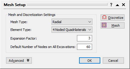
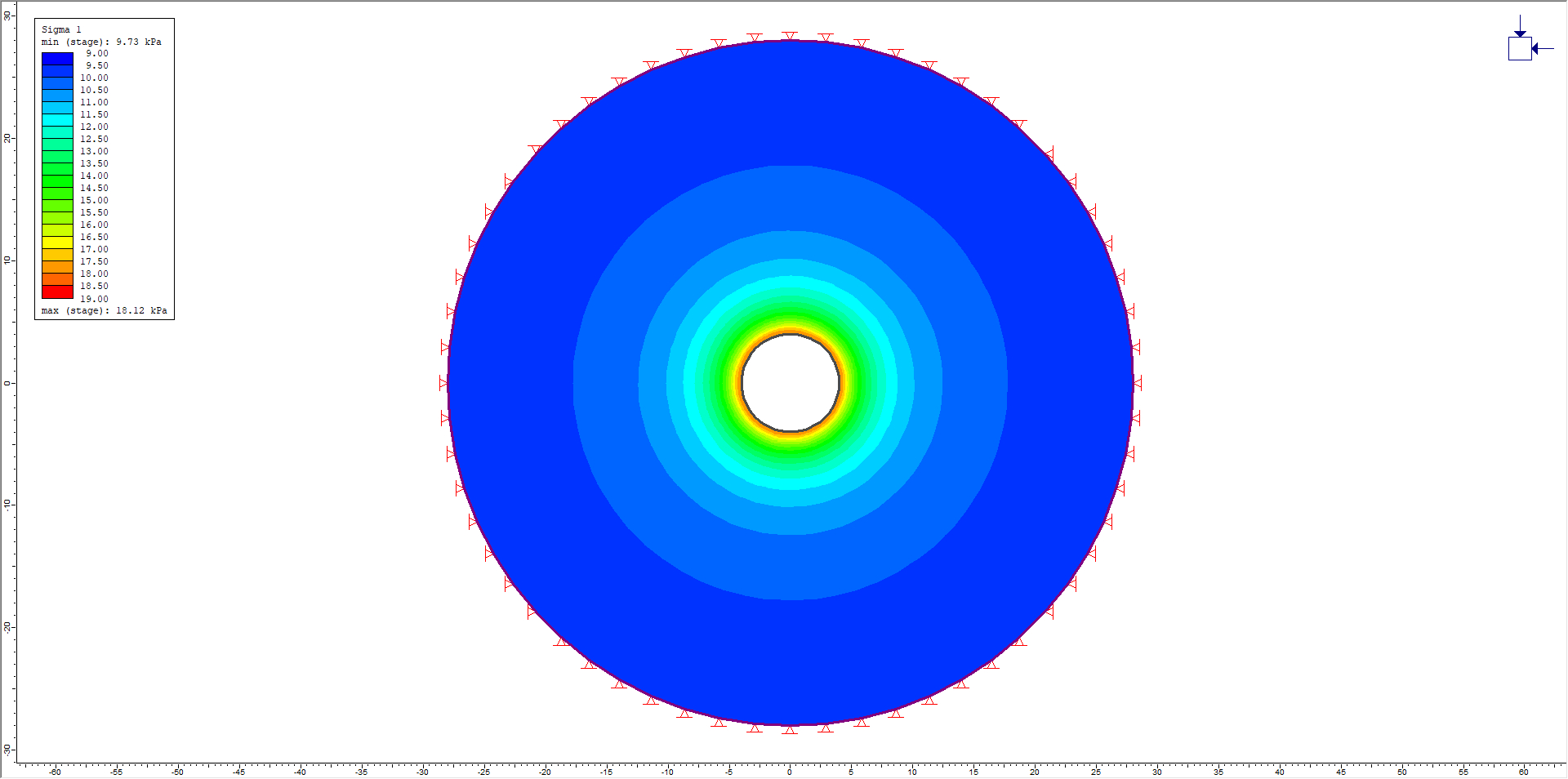
- Discretize and Mesh. The external boundary will appear when the radial mesh is generated.
- Carry out the analysis and data interpretation as before.
Plotting the displacement versus distance from the tunnel should give nearly identical results as when BOX external boundary was used. However, the displacement contours are no longer distorted and are circular at any distance from the excavation.
Also note that quadrilateral elements in conjunction with radial meshing are very efficient and give very good results.
4.2 Distance of External Boundary from Excavation
As pointed out in other tutorials, the distance of the external boundary from the excavation(s), and the boundary conditions we impose on it, are very important.
- Create another Radial mesh, as described above, except this time use an Expansion Factor of 5 (in the Mesh Setup dialog).
- Re-run the analysis and plot the displacement versus distance from the tunnel (add a query from 4,0 to 44,0).
- Export the query data to Excel for both radial mesh models (expansion factor = 3 and expansion factor = 5). Note: export query data by right-clicking on a query and selecting Copy Data or right-click on a graph and select Plot in Excel.
- In Excel, plot the query data to obtain the following figure.
The previous expansion factor of 3 was too low because displacements increase significantly when the fixed external boundary is moved further from the tunnel.
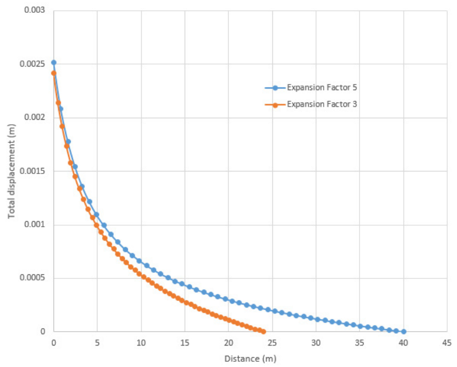
The displacements near the excavation are comparable but diverge towards the external boundary. For example, at about 18 meters from the excavation, the displacement for the Expansion Factor = 5 curve is about double the Expansion Factor = 3 curve (see above figure).
The restraining effect of a fixed external boundary should therefore always be considered. When comparing with analytical solutions, as in the RS2 verification manual, it is very important to take this into account.
One final suggested exercise:
Re-do the axisymmetric problem and move the right edge of the external boundary over to 44 meters. This gives an equivalent distance from the excavation as the plain strain model with an expansion factor of 5. Compare results with the equivalent plain strain model.
This concludes the Axisymmetric Analysis Tutorial.