3D Tunnel Simulation using Core Replacement
1.0 Introduction
In this tutorial, RS2 is used to simulate the three-dimensional excavation of a tunnel. In three dimensions, the tunnel face provides support. As the tunnel face advances away from the area of interest, the support decreases until the stresses can be accurately modelled with a two-dimensional plane-strain approach. This procedure is necessary to determine the amount of deformation prior to support installation.
A circular tunnel of radius 4m is to be constructed in Schist at a depth of 550m. The in-situ stress field has been measured with the major in-plane principal stress equal to 30 MPa, the minor in-plane principal stress equal to 15 MPa and the out-of-plane stress equal to 25 MPa. The major principal stress is horizontal, and the minor principal stress is vertical. The strength of the Schist can be represented by the Generalized Hoek-Brown failure criterion with the uniaxial compressive strength of the intact rock equal to 50 MPa, the GSI equal to 50 and mi equal to 10. To compute the rock mass deformation modulus, the modulus ratio (MR) is assumed to be 400. The support is to be installed 2m from the tunnel face.
The goal of this tutorial is to demonstrate how to model the tunnel deformation prior to support installation using the core replacement (material softening) approach.
To design a support system, the following procedure can be used:
- Determine the amount of tunnel wall deformation prior to support installation. As a tunnel is excavated, there is a certain amount of deformation, usually 35-45% of the final tunnel wall deformation, before the support can be installed. Determining this deformation can be done using either a) observed field values, or b) numerically from 3D finite-element models or axisymmetric finite-element models, or c) by using empirical relationships such as those proposed by Panet or Vlachopoulos and Diederichs.
- Using the core replacement technique, determine the modulus reduction sequence that yields the amount of tunnel wall deformation at the point of and prior to support installation. This is the value determined in step 1 (Core Replacement Part 1 Model)
- Build a model that relaxes the boundary to the calculated amount in step 2. Add the support and determine whether a) the tunnel is stable, b) the tunnel wall deformation meets the specified requirements, and c) the tunnel lining meets certain factor of safety requirements. If any of these conditions are not met, choose a different support system and run the analysis again (Core Replacement Part 2 Model)
2.0 Construct the Model
2.1 Project Settings
Start with a new RS2 project file.
- Select: Analysis > Project Settings

- Under the Units tab, define the units as “Metric, stress as MPa.”
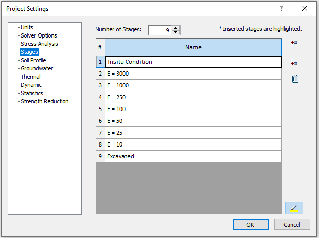
- Under the Stages tab, change the Number of stages to 9 (see following figure). Fill in the stage names as shown below.
- Close the dialog by clicking OK.
| # | Name |
| 1 | Insitu Condition |
| 2 | E = 3000 |
| 3 | E = 1000 |
| 4 | E = 250 |
| 5 | E = 100 |
| 6 | E = 50 |
| 7 | E = 25 |
| 8 | E = 10 |
| 9 | Excavated |
2.2 Geometry

Now enter the circular tunnel.
- Select: Boundaries > Add Excavation

- Right-click the mouse and select the Circle option from the popup menu.
- Select the Center and radius option, enter Radius = 4 and enter Number of Segments = 96 and select OK.
- Enter the circle center as (0,0) in the prompt line and the circular excavation will be created.
- Select Zoom All (or press the F2 function key) to zoom the excavation to the center of the view.
Now let’s create the external boundary. In RS2, the external boundary may be automatically generated, or user-defined. Let’s use one of the ‘automatic’ options:
- Select: Boundaries > Add External

- In the Create External Boundary dialog, use set Boundary Type = Box and Expansion Factor = 5. Select OK, and the external boundary will be automatically created.
The boundaries for this model have now been entered.
2.3 Materials
![]()
- Select: Properties > Define Materials

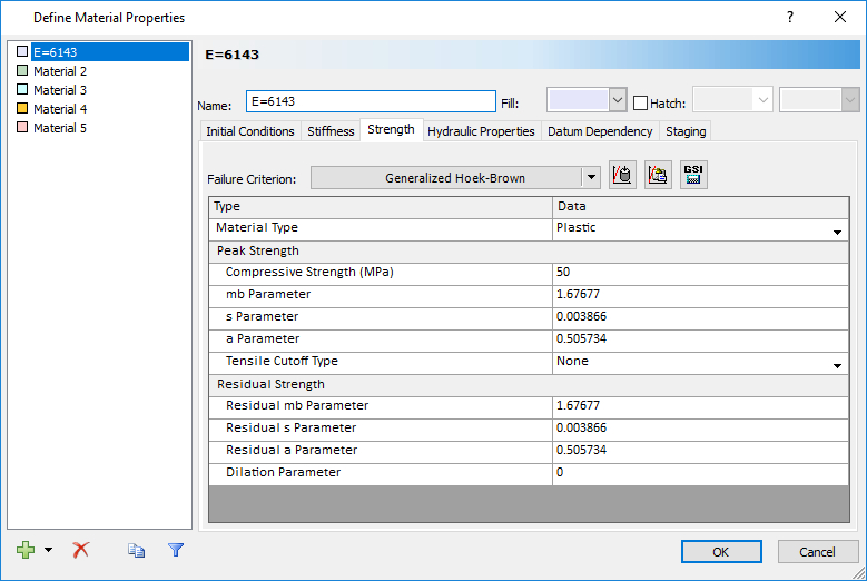
- For Material 1, under the Strength tab, change the Failure Criterion to Generalized Hoek-Brown and the Material Type to Plastic.
- Now define the strength parameters and the Young’s Modulus using the GSI calculator. Click the GSI calculator
 button:
- In the GSI calculator dialog, set the uniaxal compressive strength of the intact rock equal to 50 MPa, the GSI equal to 50 and mi equal to 10. To compute the rock mass deformation modulus, set the modulus ratio (MR) to 400.
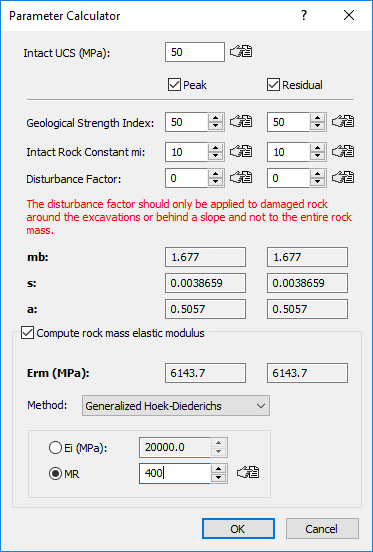
- Press the OK button. The material properties dialog should now be updated with the new strength and modulus values.
- In the GSI calculator dialog, set the uniaxal compressive strength of the intact rock equal to 50 MPa, the GSI equal to 50 and mi equal to 10. To compute the rock mass deformation modulus, set the modulus ratio (MR) to 400.
- Change the Name of Material 1 to E=6143. The dialog should look as follows:
- Click on the Material 2 tab and change the name to E=3000. In the Initial Condition tab, change the Initial Element Loading to None. In the Stiffness tab, change the Young’s Modulus to 3000 MPa.
- Now follow the same procedure and set the Young’s modulus of Materials 3 through 8 to 1000, 250, 100, 50, 25, and 10 MPa respectively. Change the names to reflect the value of the modulus. Make sure that the Initial Element Loading for Materials 3 thru 8 is set to None.
- Click OK when done.
The first material, with modulus 6143 MPa and Generalized Hoek-Brown failure criterion, is the in-situ rock mass. Materials 2 through 8 will be used inside the excavation (excavation core). The core material is progressively replaced over several stages. This replacement, along with the modulus reduction, allows the boundary to progressively deform. In each of the eight stages, the material inside the excavation is replaced by a material with zero internal stress (i.e. Initial Element Loading = None) and with a lower modulus than the proceeding stage. In the final stage, the material inside the excavation is removed. This process models the advancement of the tunnel face. Each stage (and corresponding core modulus) represents some distance from the tunnel face, either in front of or behind the face. The final excavated stage represents the deformed state far away from the tunnel face, at a distance where the face has no influence on stresses or displacements. What’s left is determining the correspondence between core modulus and distance from the tunnel face, specifically, the modulus sequence that yields the deformation at the support installation distance. The support installation distance being the distance between the tunnel face and where the support is installed.
To determine the correspondence between core modulus and distance from the tunnel face, the relationship between tunnel wall deformation and distance from the tunnel face must be known. Knowing the relationship between tunnel wall displacement and distance from the tunnel face and knowing the relationship between core modulus and tunnel wall displacement, the relationship between core modulus and distance from the tunnel face can then be determined. Knowing this relationship allows the calculation of the modulus reduction sequence that gives the tunnel wall displacement prior to support installation.
2.4 Core Replacement Technique
- Select: Zoom Excavation
 on the toolbar
 - Select: Properties > Assign Properties
- Make sure the Stage 2 tab, E=3000, is selected (at the bottom left of the view).
- Select the “E=3000” button in the Assign dialog.
- Click the left mouse button inside the tunnel. The material inside the tunnel should change to green, the color representing the E=3000 material.
- Change to Stage 3, E=1000, by clicking the stage tab at the bottom of the screen.
- Select the “E=1000” button in the Assign dialog.
- Click the left mouse button inside the tunnel. The material inside the tunnel should change to light blue, the color representing the E=1000 material.
- Change to Stage 4, E=250.
- Select the “E=250” button in the Assign dialog.
- Click the left mouse button inside the tunnel.
- Change to Stage 5, E=100.
- Select the “E=100” button in the Assign dialog.
- Click the left mouse button inside the tunnel.
- Change to Stage 6, E=50.
- Select the “E=50” button in the Assign dialog.
- Click the left mouse button inside the tunnel.
- Change to Stage 7, E=25.
- Select the “E=25” button in the Assign dialog.
- Click the left mouse button inside the tunnel.
- Change to Stage 8, E=10.
- Select the “E=10” button in the Assign dialog.
- Click the left mouse button inside the tunnel.
- Change to Stage 9, Excavated.
- Select the “Excavate” button at the bottom of the Assign dialog.
- Click the left mouse button inside the tunnel. The material inside the excavation should now be removed.
- Close the Assign dialog by clicking on the X in the upper right corner of the dialog.
Now select Stage 1 – the in-situ condition stage. Turn on the minimum data tips mode using the following command. - Select: View > Data Tips > Minimum
Hover the mouse inside the excavation. After a second, a data tip should appear: 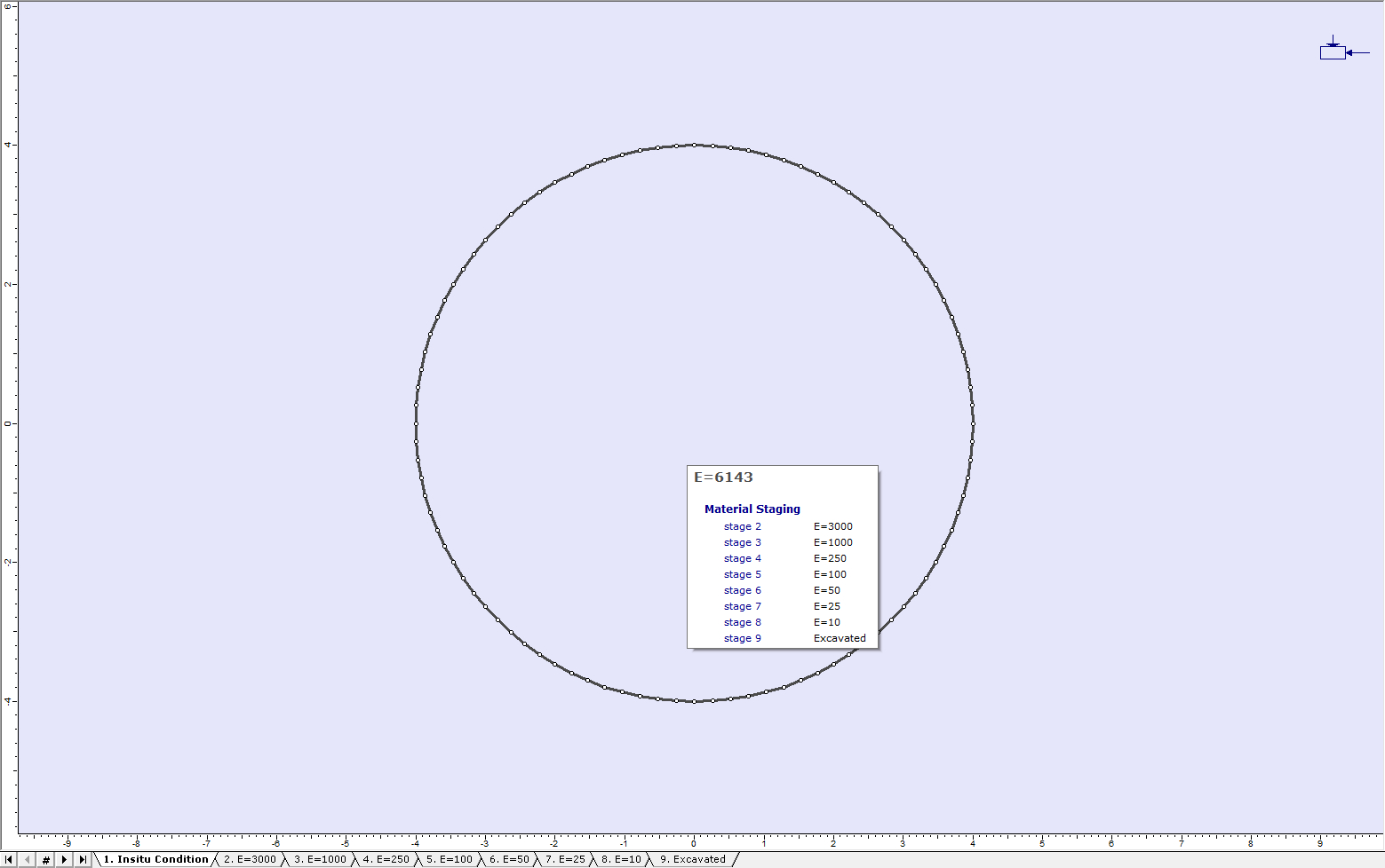
Notice that the data tip shows all the materials inside the excavation as a function of stage.
Let’s run the analysis.
2.5 Mesh
![]()
- Select: Mesh > Mesh Setup

- In the mesh setup dialog, ensure the Element Type is 6 Noded Triangles.
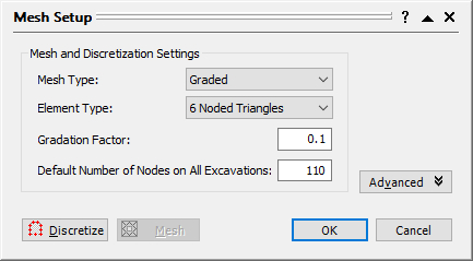
- Click the Discretize button and then the Mesh button. Click OK to close the dialog.
2.6 Field Stress

Field Stress determines the initial in-situ stress conditions, prior to excavation.
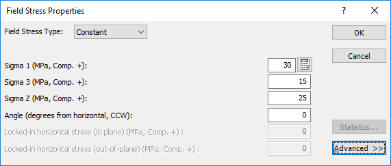
- Select: Loading > Field Stress

- Select Field Stress Type = Constant.
- Enter Sigma 1 = 30, Sigma 3 = 15, Sigma Z = 25, Angle = 0, and select OK.
- Select: File > Save
 . Name the file as 3D Tunnel Simulation using Core Replacement (Part 1).
 - Select: Analysis > Compute

3.0 Results and Discussion
- Select: Analysis > Interpret

The maximum stress, Sigma 1 for Stage 1 will be displayed. Notice that there is no variation of stress and that the stress (30 MPa) is equal to the major in-situ field stress. This is expected since in the first stage the material inside and outside the tunnel boundary is the in-situ E=6143 material.
- Select: Zoom Excavation on the toolbar
- Change the contours to plot Total Displacement using the pull-down menu in the toolbar.
The model for Stage 1 will look like this:
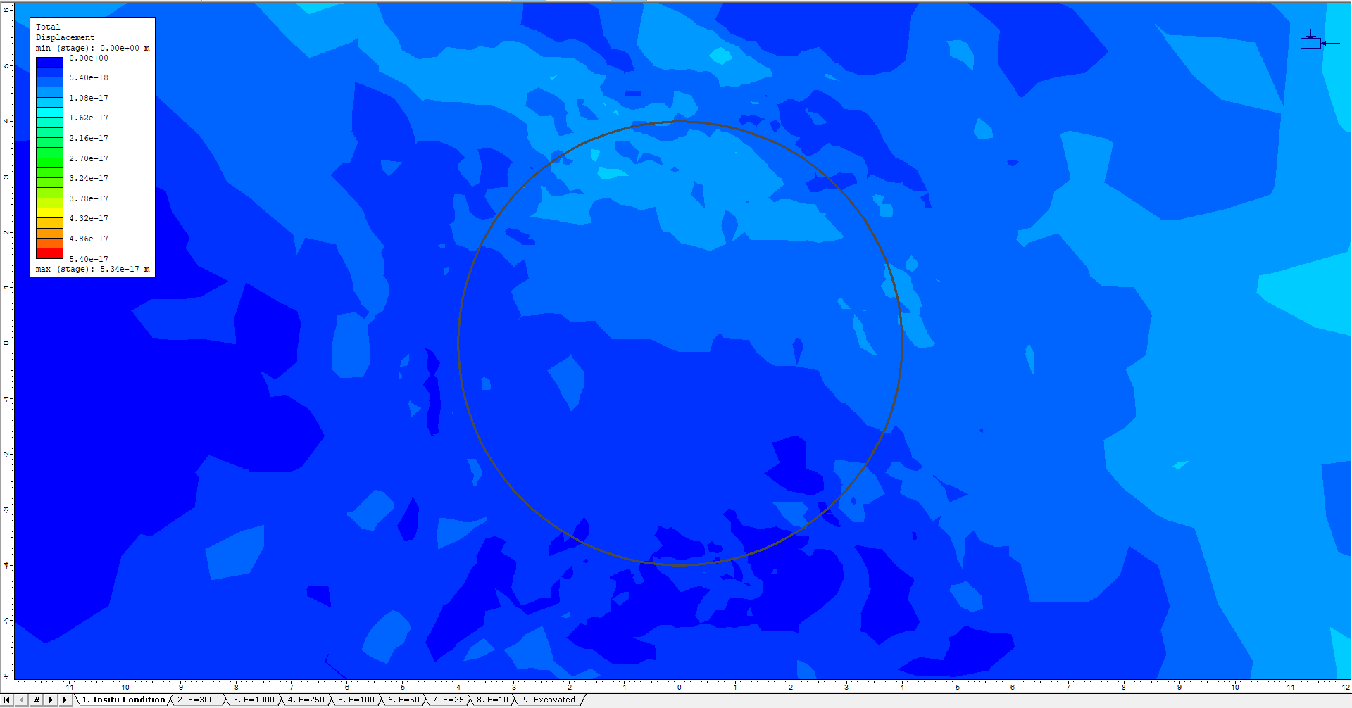
There is essentially no displacement in the first stage. Now click through the stages. An increase in deformation is visible around the tunnel as the core material is replaced and softened (modulus reduced).
3.1 Step 1: Computing tunnel deformation before support installation using the Vlachopoulos and Diederichs method
To compute the tunnel deformation at the point of support installation, use the empirical relationship developed by Vlachopoulos and Diederichs. To use this method, information from the finite element analysis is required: a) the maximum tunnel wall displacement far from the tunnel face, and b) the radius of the plastic zone far from the tunnel face.
Both values can be computed from a plane strain analysis with zero internal pressure inside the excavation. In the model constructed in this tutorial, the results from stage 9 are used since the material inside the excavation is completely removed in this stage.
Switch to the last stage (Stage 9). Look at the bottom of the legend. The maximum displacement for this stage is approximately 0.05 m. This is the value of maximum wall displacement far from the tunnel face. The location of this displacement is in the roof and floor of the excavation. The location of this displacement is important since any comparisons of displacement for various core moduli must be made at the same location.
- To determine the radius of the plastic zone, click Display Yielded Elements
 .
.
Several crosses are visible and represent elements in the finite element analysis that have failed. - Zoom Out so that the entire extent of failed points is visible (see below).

The extent of this failed zone represents the extent of the plastic zone around the tunnel. To determine the radius of the plastic zone, use either the measuring tool or the dimensioning tool to measure the distance from the center of the tunnel to the perimeter of the yielded/plastic zone. This tutorial uses the measuring tool:
- Select: Tools > Add Tool > Measure
- Select (0, 0) as the location to measure from. Use the mouse to extend the measuring line vertically until the edge of the yield zone is reached. Click here to select.
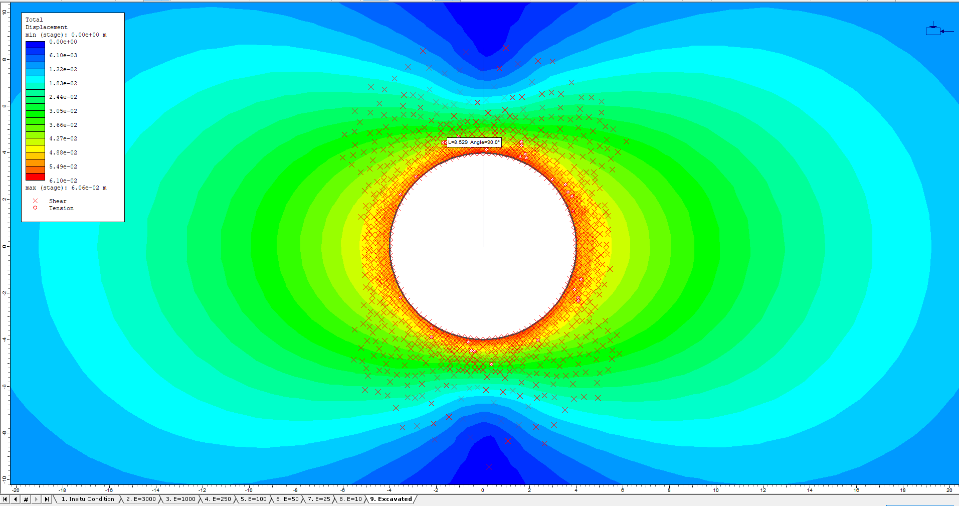
As seen above, the radius of the plastic zone is approximately 8.5 m.
3.1.1 Computing displacement prior to support installation using the Vlachopoulos and Diederichs Method
The following plot was created using the Vlachopoulos and Diederichs equations (Vlachopoulos and Diederichs, 2009). The equations can also be found in the Kersten Lecture, appendix 1 (Hoek et. al., 2008). Using this plot, it is possible to estimate the amount of closure prior to support installation if the plastic radius and displacement far from the tunnel face are known.
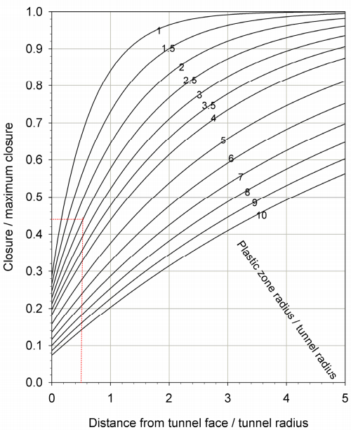
For our problem, Rp=8.5m, Rt=4m, X=2m, and umax=0.061m. The Distance from tunnel face/tunnel radius = 2/4 = 0.5. The Plastic zone radius/tunnel radius = 8.5/4 = 2.1. From the above plot this gives Closure/max closure approximately equal to 0.49. Therefore the closure equals (0.49)*(0.061) = 0.030 m.
As computed above, the tunnel roof displaces 0.030m before the support is installed.
3.2 Step 2: Determining the core modulus
The next step is to determine the core modulus that yields a displacement of 0.030m in the roof of the tunnel. It is important to maintain the same location as is used to determine umax, since the location of maximum displacement can change depending on the magnitude of the internal pressure. This can be seen in this model as larger core moduli produce larger displacement in the sidewall while smaller core moduli produce larger displacements in the roof and floor.
To determine the internal pressure that yields a 0.030m roof displacement, plot the displacement versus stage for a point on the roof of the excavation.
- Ensure Total Displacement is selected as the data type.
3.2.1 Graphing Displacement in the Roof of the Excavation
To create the graph:
- Select: Graph > Graph Single Point vs.. Stage
- When asked to enter a vertex, type in the value 0, 4 for the location and press Enter. This is a point on the roof of the excavation.
- The Graph Query Data dialog will appear:
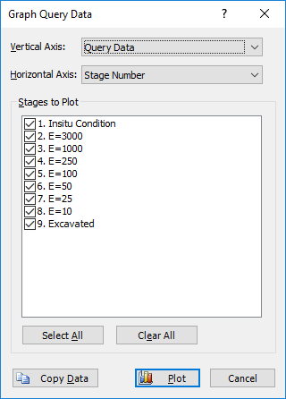
- Press the Plot button. The following figure shows the plot generated by the program. This is a plot of displacement versus stage for a point in the roof of the tunnel.
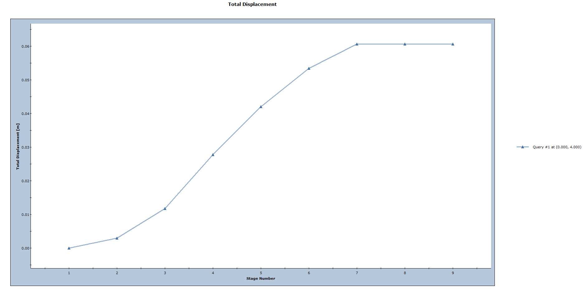
- Right-click in the plot and choose Sampler > Show Sample. Move the sampler by moving the mouse with the left mouse button. Move the sampler until the displacement value on the right side of the plot is equal to 0.030m.

This plot shows that in stage 4, the wall displacement in the roof of the tunnel is approximately 0.030m. This represents a 3-stage material replacement and reduction of core modulus from E=6143(insitu), to 3000, 1000 and finally 250 MPa.
3.2.2 Creating a convergence confinement graph in Excel
To create a convergence confinement graph (plots displacement versus core modulus), export the above graph to Microsoft Excel™.
- Right-click in the graph and choose the Plot in Excel option.
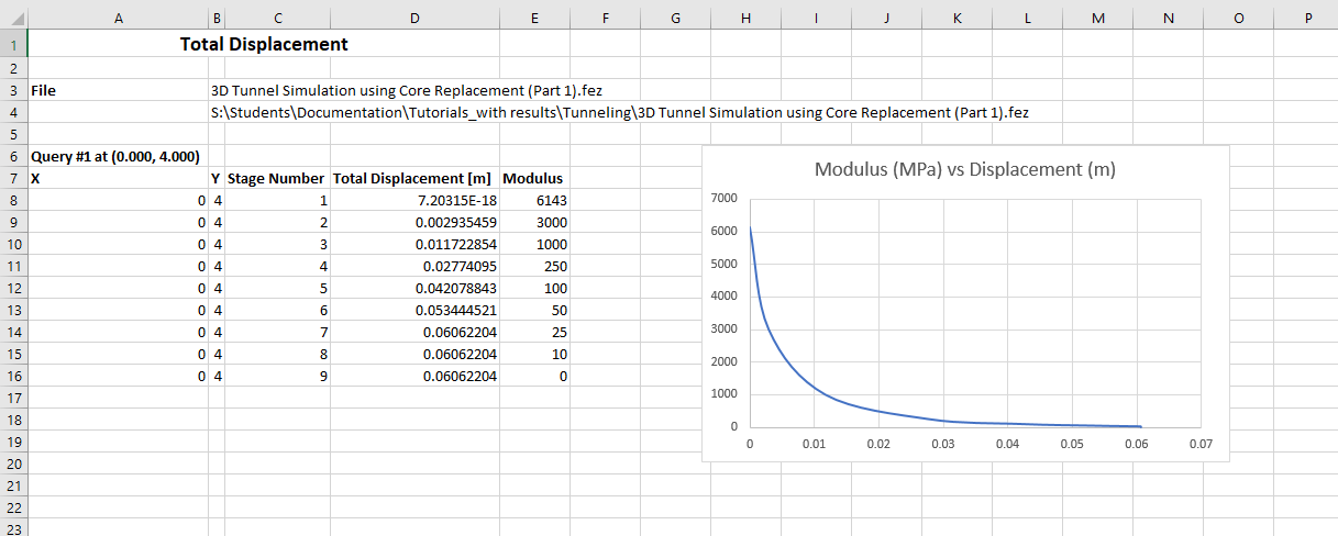
Excel will launch with a plot of stage number versus displacement. The plot can be easily changed to show the stage number data to the core modulus. A sample of the Excel file for this example is included in the Tutorials folder with the RS2 data files.
The following image shows the convergence-confinement plot in Excel for this example. The plot shows that modulus reduction to 250MPa yields the tunnel wall displacement computed above for the point of support installation (0.030m).
Steps 1 and 2 as defined in the Problem section at the beginning of this tutorial have been completed; lets proceed by defining the support system.
- From Interpret, switch back to the RS2 Model
 program.
4.0 Model: With Support
We will now use the 9-stage model created above and modify it to create the support design.
4.1 Project Settings
- Select Analysis > Project Settings and select the Stages Tab.
- Use the Delete Stages button to delete stages 5,6,7, and 8.
- Change the name of stage 5 from Excavated to Support Installed.
The dialog should look like: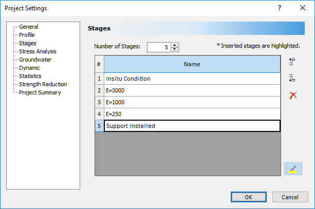
- Close the dialog by clicking OK.
- Make sure the Stage 5, Support Installed stage tab is selected. Click the Zoom Excavation button on the toolbar.
It is important that we keep all the core softening stages up to the stage that represents support installation. This is because the replacement and softening of the core material in stages 2 and 3 affect the final displacement result. These stages directly influence the stress path and displacement of the material around the excavation.
4.2 Setting the Reinforced Concrete Liner Properties

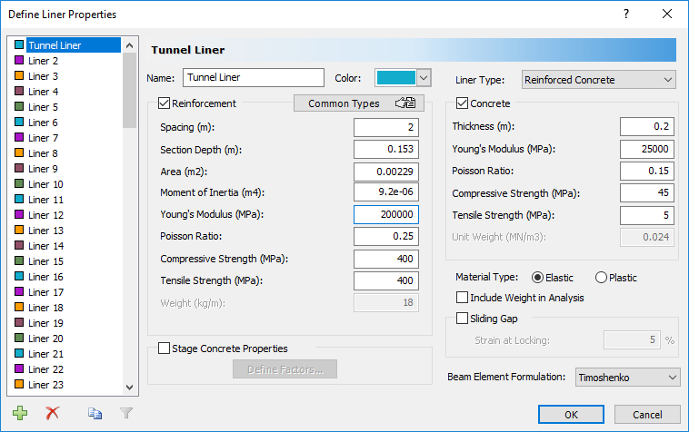
Now define the liner properties. The properties correspond to a 200 mm thick layer of concrete reinforced with W150X18 I-beams spaced at 2-meter intervals along the tunnel axis.
- Select: Properties > Define Liners
- Change the Name of the liner to Tunnel Liner
- Change the Liner Type to Reinforced Concrete
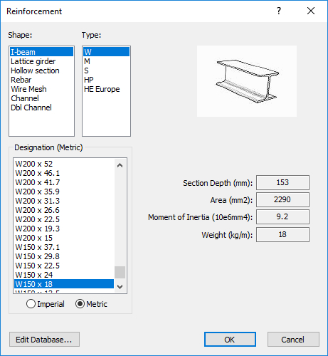
- Click on the Common Types button. In the Reinforcement database dialog:
- Select an I-beam from a list of standard reinforcement types.
- Select the W150 x 18 I-beam.
- Click OK, and the I-beam reinforcement properties will be automatically loaded into the Define Liner Properties dialog.
- In the Define Liner Properties dialog, for the Reinforcement, enter a spacing of 2m.
- Enter the properties for the concrete.
- Thickness=0.2m
- Modulus=25000MPa
- Poisson Ratio=0.15
- Compressive Strength=45MPa
- Tensile Strength=5MPa.
- Click OK to save the input and exit the dialog.
The liner properties dialog should look like:
4.3 Adding a Reinforced Concrete Liner to the Tunnel
![]()
Let’s line the tunnel with the liner defined above. First make sure that Stage 5, the Support Installed stage, is selected.
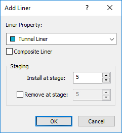
- Select: Support > Add Liner
- In the Add Liner dialog, select Tunnel Liner as the Liner Property and set the liner to install at stage = 5. Select OK.
- Click and hold the left mouse button and drag a selection window which encloses the entire excavation. Release the left mouse button. Notice that all excavation line segments are selected.
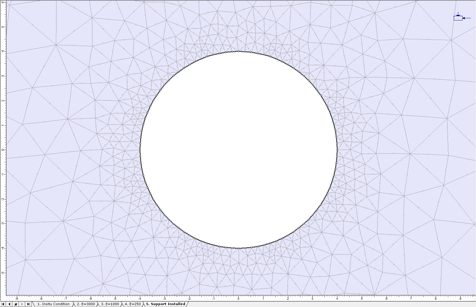
- Right-click the mouse and select Done Selection, or just press the Enter key. The entire tunnel will now be lined, as indicated by the thick blue line segments around the excavation boundary (see below).

Click through the stages. Notice how the color of the liner changes from light blue in stages 1 through 4 to dark blue in stage 5. This indicates that the liner is being installed in stage 5.
The model is ready for analysis.
5.0 Compute
Before analyzing the model, save it as a new file called 3D Tunnel Simulation using Core Replacement (Part 2).fez (make sure to select Save As and not Save, or it will overwrite the internal pressure reduction file).
- Select: File > Save As to save the model
- Save the file as 3D Tunnel Simulation using Core Replacement (Part 2).fez.
- Select: Analysis > Compute
The RS2 Compute engine will proceed in running the analysis.
6.0 Results and Discussion: With Support
From Model, switch to the Interpret program.
- Select: Analysis > Interpret
- If any other files are loaded in the Interpret program (i.e. the CoreSoftening.fez file), close them. Click on the tab at the bottom of the program window associated with the file and use the File > Close menu option to close the file.
- Make sure the Stage 5 tab is selected and zoom in on the excavation.
6.1 Support Capacity Diagrams
Support capacity diagrams give the engineer a method for determining the factor of safety of a reinforced concrete liner. For a given factor of safety, capacity envelopes are plotted in axial force versus moment space and axial force versus shear force space. Values of axial force, moment, and shear force for the liner are then compared to the capacity envelopes. If the computed liner values fall inside an envelope, they have a factor of safety greater than the envelope value. So, if all the computed liner values fall inside the design factor of safety capacity envelope, the factor of safety of the liner exceeds the design factor of safety.
- Select: Graph > Support Capacity Plot

The Support Capacity Plot dialog allows the user to choose the support element (i.e. liner type), the number of envelopes, and the stages from which the liner data is taken. - Increase the Number of Envelopes to 3.
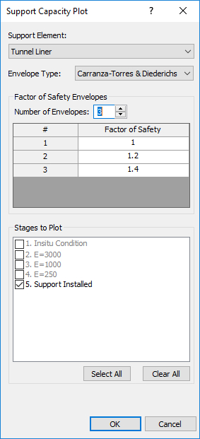
- Click OK.
The following plot is generated. The dark red lines represent the capacity envelopes for the 3 factors of safety (1, 1.2, 1.4).
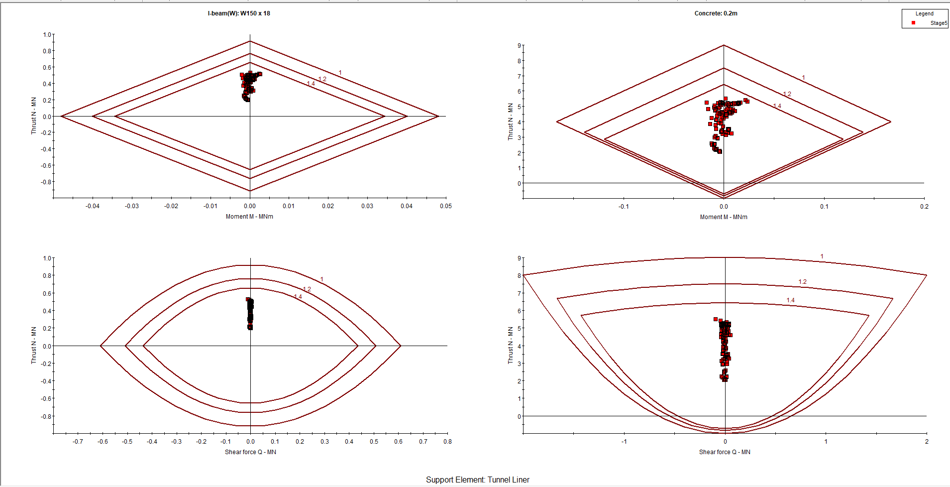
Notice that all the data points fall within the factor of safety=1.4 envelope, on all four plots. This means that the support system chosen has a factor of safety greater than 1.4.
Note about determining the final core modulus:
In this example, the required core modulus, which gives the displacement required at the point of support installation, happens to be exactly equal to one of the original modulus values chosen for the initial reduction sequence (i.e. 250 MPa). In general, this will not be the case. That is, the required core modulus will probably lie between two of the values chosen for the initial modulus reduction sequence. If this occurs:
- Use the convergence-confinement graph to determine the required core modulus at the point of support installation, as discussed earlier in this tutorial.
- Then either insert a new stage of core replacement, with the required modulus value, or simply use the nearest stage with a HIGHER modulus value and lower the material modulus at this stage to the required value (e.g. if the required modulus is 350 MPa, but the initial sequence goes from 500 to 250, then change the 500 to 350).
- Re-run the analysis and check if the new modulus value does in fact give the desired displacement at the point of support installation. It should be close. If not, then repeat steps 1 to 3 until the required modulus value is determined.
This concludes the 3D Tunnel Simulation Tutorial.
7.0 References
Hoek, E., Carranza-Torres, C., Diederichs, M.S. and Corkum, B. (2008). Integration of geotechnical and structural design in tunnelling – 2008 Kersten Lecture. Proceedings University of Minnesota 56th Annual Geotechnical Engineering Conference. Minneapolis, 29 February 2008, 1-53.
Vlachopoulos, N. and Diederichs, M.S. (2009). Improved longitudinal displacement profiles for convergence-confinement analysis of deep tunnels. Rock Mechanics and Rock Engineering, 42(2), 131-146.