Drawdown Analysis for Slope
1.0 Introduction
In this tutorial, two different methods of modelling the staged drawdown of ponded water against a slope are examined and an SSR slope stability analysis is performed. The drawdown is implemented in two ways: 1) by lowering the water table, and 2) by running a finite element groundwater analysis with changing boundary conditions.
2.0 Constructing the Model: Drawdown with Piezometric Lines
- Select: File > Recent Folders > Tutorial Folder
- Open the Drawdown Analysis for Slope (initial) file.
The geometry, material properties, and project settings have already been specified for this model.
2.1 Piezometric Lines

In the first stage, there will be 10 m of ponded water at the base of the slope. In the second stage, the ponded water will drop down 5 m.
Ensure Stage 1 is selected.
- Select: Boundaries > Add Piezometric Line

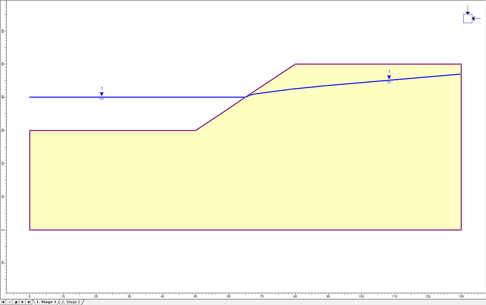
- Enter the following coordinates: (0, 40), (65, 40), (66.35, 40.6), (67.7, 41), (78.3, 42.4), (89.4, 43.5), (130, 47). Press Enter
- In the “Assign Piezometric Line to Materials” dialog, select Soil 1
- Click OK.
The model should now look like this:
In the second state, the ponded water will be dropped by 5 m.
- Click on the tab for Stage 2.
- Select: Boundaries > Add Piezometric Line
- Enter the following coordinates: (0, 35), (57.5, 35), (58.7, 35.8), (60.1, 36.3), (65.3, 37.3), (76.6, 39), (93.5, 41.1), (110, 43), (130, 45). Press Enter.
- Select Soil 1 in the ‘Assign Piezometric Line to Materials’ dialog and click OK. The model should now look like this:
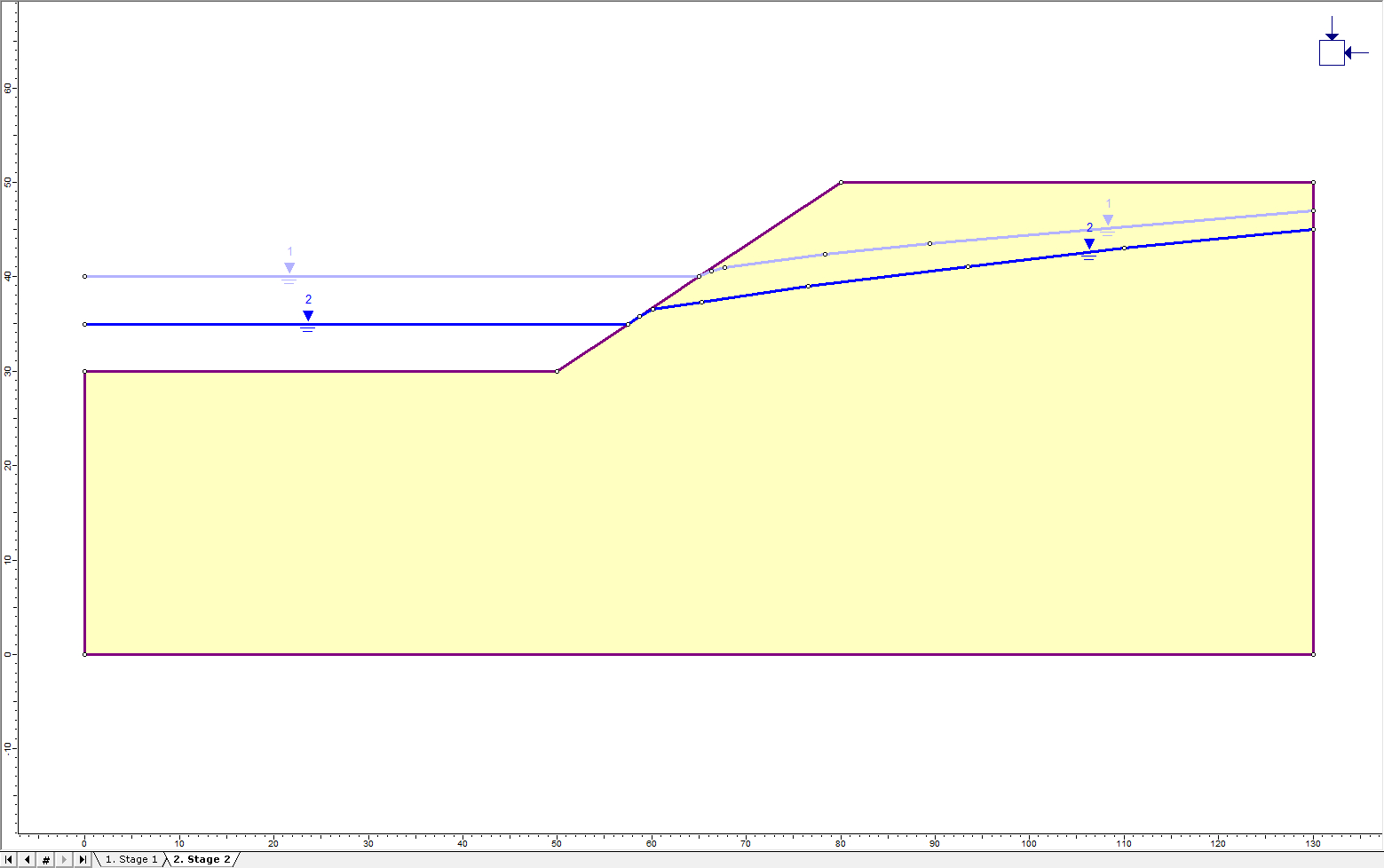
Notice that the new water table (piezo 2) has superseded the old water table (piezo 1).
- Go back to Stage 1.
Stage 1 is the same as Stage 2; the active water table is piezo 2, and piezo 1 is inactive.
The piezo lines now need to be staged:
- Select: Properties > Define Hydraulic

- Select the Staging tab. Check the box for Stage Hydraulic Properties.
- For Stage 1, choose Piezo #1 and for Stage 2, choose Piezo #2.
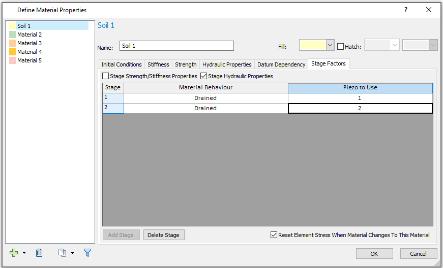
- Click OK to close the dialog. Now click through the stages; piezo 1 is active in Stage 1 and piezo 2 is active in Stage 2.
2.2 Ponded Water Load
![]()
In this model, there is ponded water at the left side of the model. This applies a stress to the soil surface due to the weight of the water. To account for this:
- Select: Loading > Ponded Water Loads > Add Ponded Water Load
- Select the Stage Load check box.
- Click the Stage Total Head button.
- In Stage 1, the y-coordinate of the water table is 40 m. Enter a Total Head of 40 m.
- In Stage 2, the water table is at 35 m, so change the Total Head for Stage 2 to 35 m as shown:
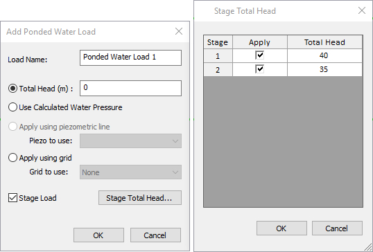
- Click OK and then click OK to close the ‘Add Ponded Water Load’ dialog.
Select the boundary segments on which to apply the ponded water load: - Select the horizontal surface between (0,30) and (50,30) as well as the two segments on the slope below piezo 1.
The model for Stage 1 should look like this:
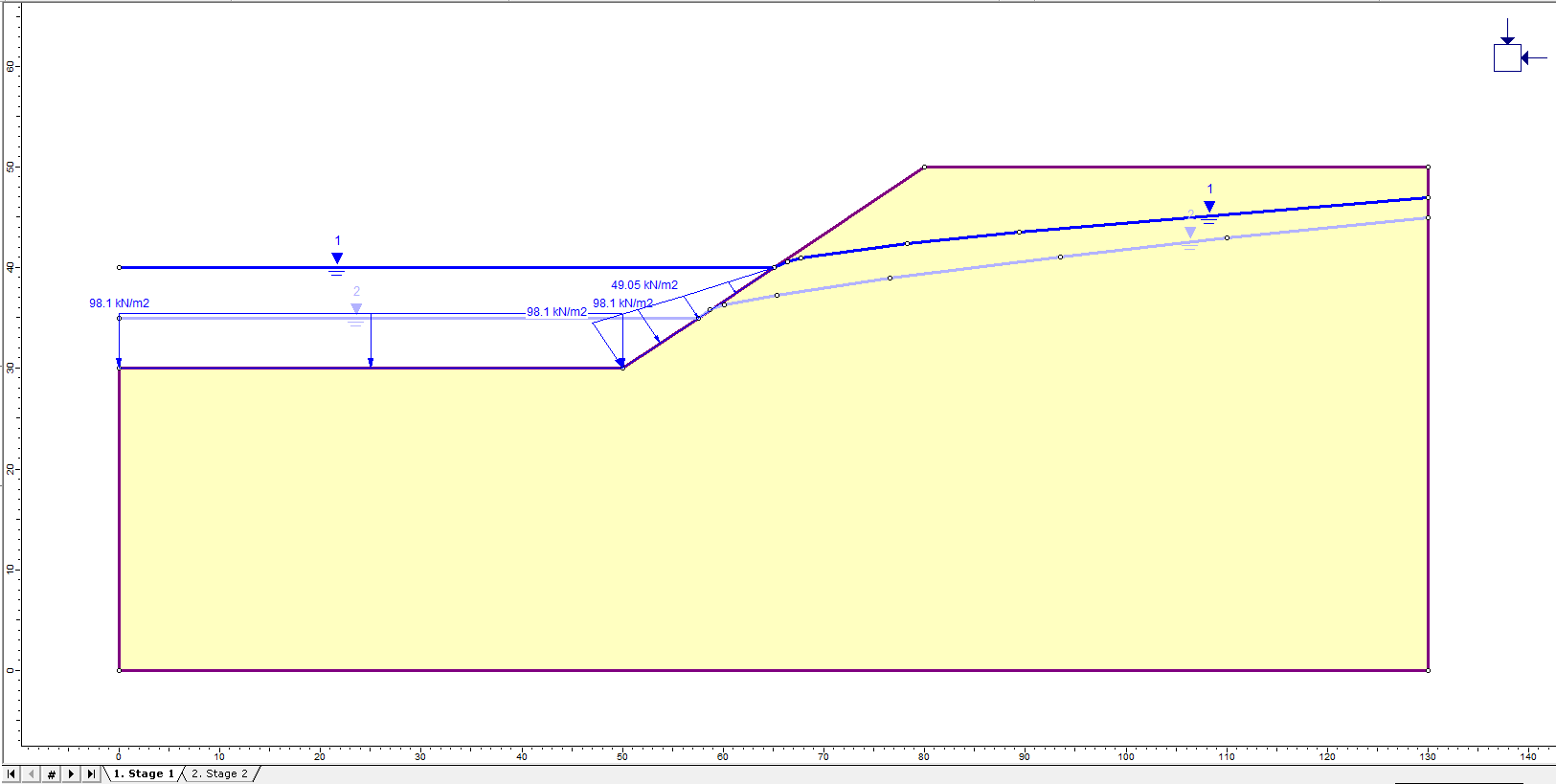
Due to the weight of the water in Stage 1, the load ranges from 0 to 98.1 kPa. In Stage 2, the depth of ponded water is reduced by half, so the maximum load is 49.05 kPa.
2.3 Mesh

- Select: Mesh > Mesh Setup

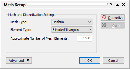
- Set the Mesh Type as Uniform, the Element Type to 6 Noded Triangles, and the Approximate Number of Mesh Elements to 1500.
- Generate the mesh by selecting the Discretize button, then the Mesh button. Click OK to close the Mesh Setup dialog.
The model definition is now complete. - Select: File > Save As
 to save the model.
3.0 Compute: Drawdown with Piezometric Lines
- Select: Analysis > Compute

Because RS2 is performing a Shear Strength Reduction analysis, the model will take several minutes to run.
4.0 Results and Discussion: Drawdown with Piezometric Lines
- Select: Analysis > Interpret

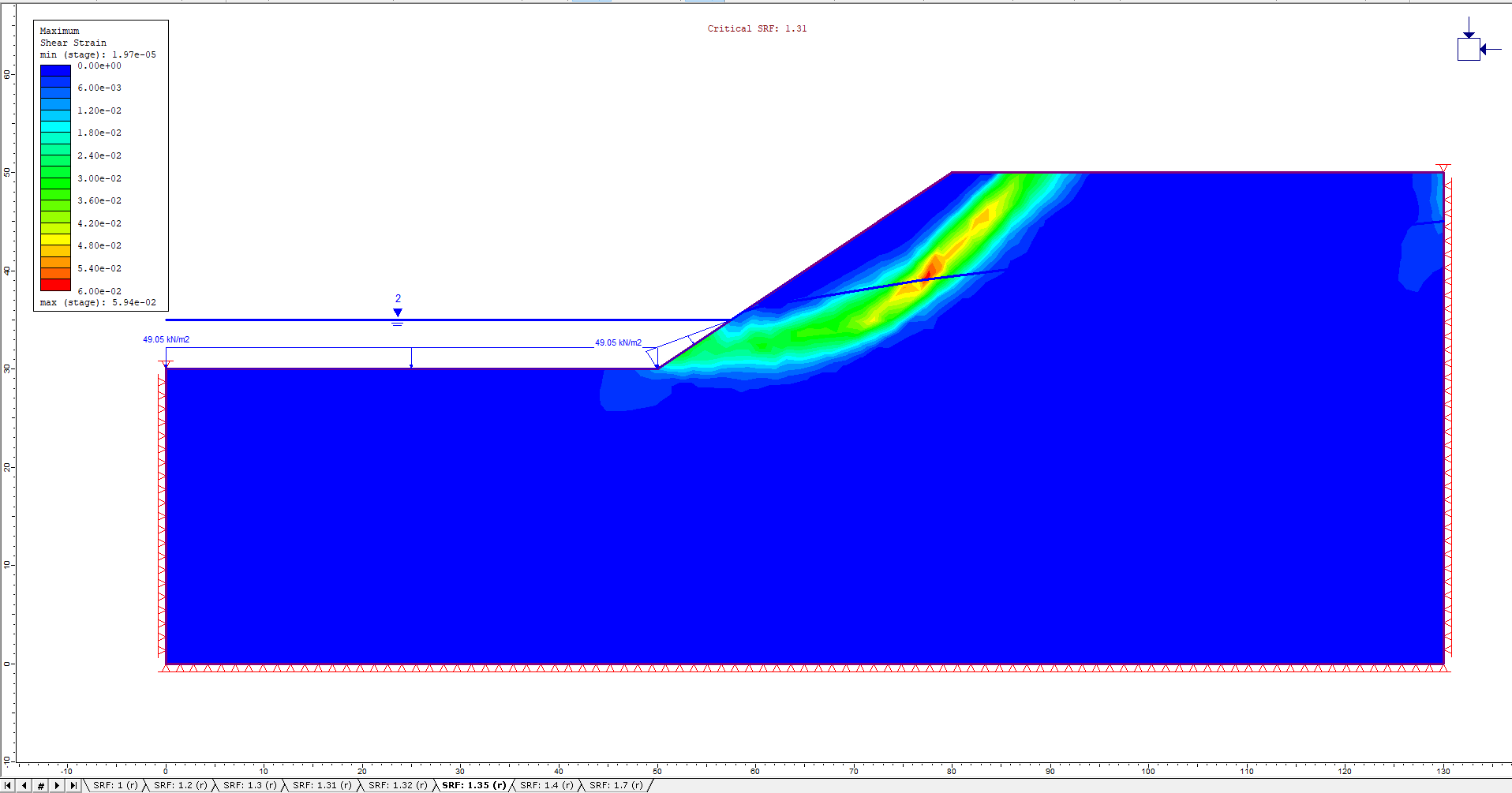
The Shear Strength Reduction analysis is only performed on the last stage of the model, so the maximum shear strain for the critical strength reduction factor for the second stage is displayed:
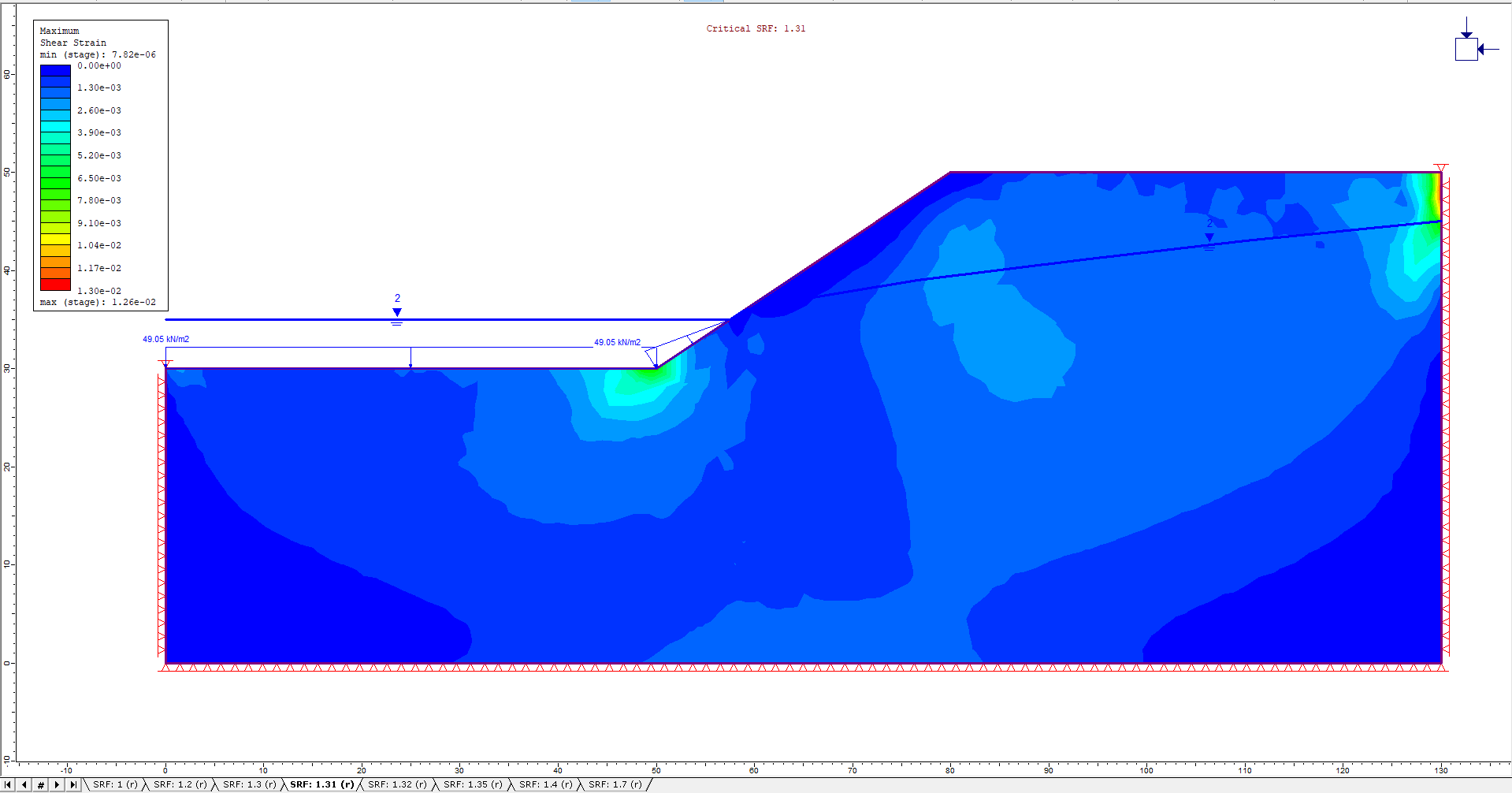
Click the tab for SRF: 1.35 to better view the critical failure surface.
To view the stage data prior to the SSR analysis:
- Select: Data > Stage Settings
- Set the Reference Stage to Not Used and the Visible Stage to Stage 1.
- Click OK. The maximum shear strain in stage 1 will now be displayed.
- Change the plot to Pore Pressure using the drop-down menu in the toolbar
- The pore pressure due to the water table in Stage 1 is now visible.
- Click the tab for Stage 2 to see how the pore pressure decreases as the water table is lowered.
5.0 Drawdown with Finite Element Groundwater Analysis
The same analysis can be performed using finite elements to compute the pore pressures in the model instead of Piezometric lines.
Go back to the RS2 Model program.
- Select: Analysis > Project Settings

- Select the Groundwater tab
- Change the method to Steady State FEA. Click on the “...” next to Steady State Settings to ensure that the values are the same as below. Leave all other options as shown:
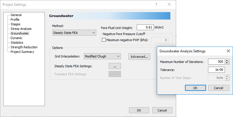
- Click OK to close the dialog.
- Right-click on the Piezometric Lines entity in the Visibility Tree on the left side of the screen. Select "Delete from Model" to remove both piezometric lines.
5.1 Groundwater Boundary Conditions

Ensure Stage 1 is selected.
- Select: Groundwater > Set Boundary Conditions

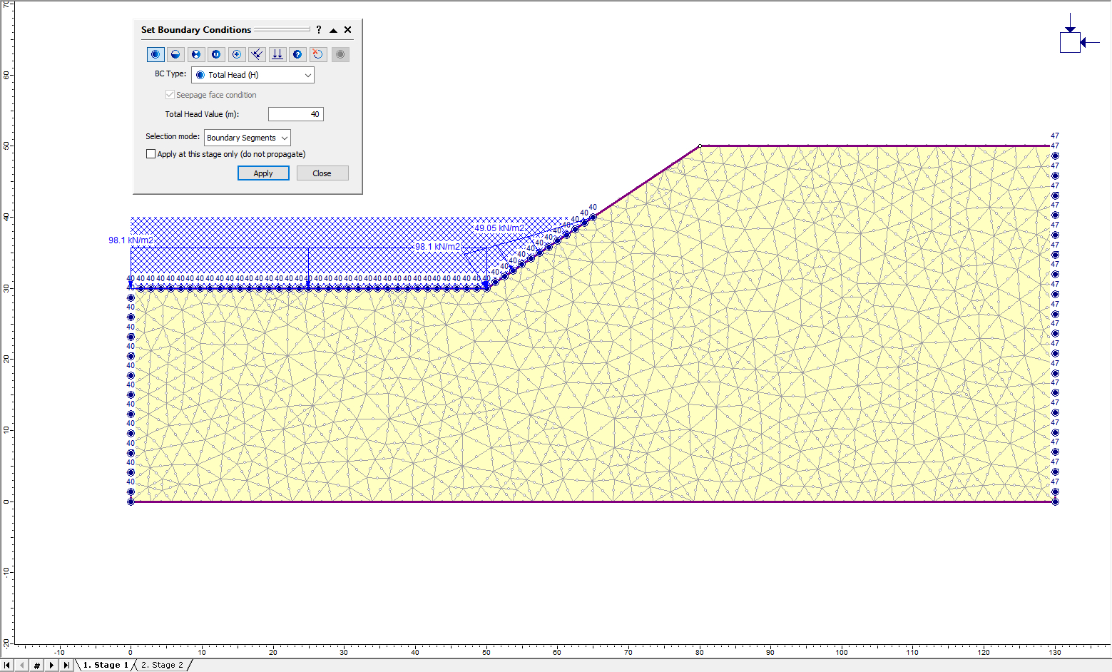
- For the BC Type, choose Total Head. Set the Total Head Value to 47 m.
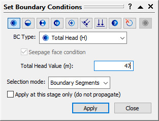
- Use the mouse to select the right vertical boundary of the model. Click Apply in the dialog. The right side of the model should display a total head boundary condition as shown:
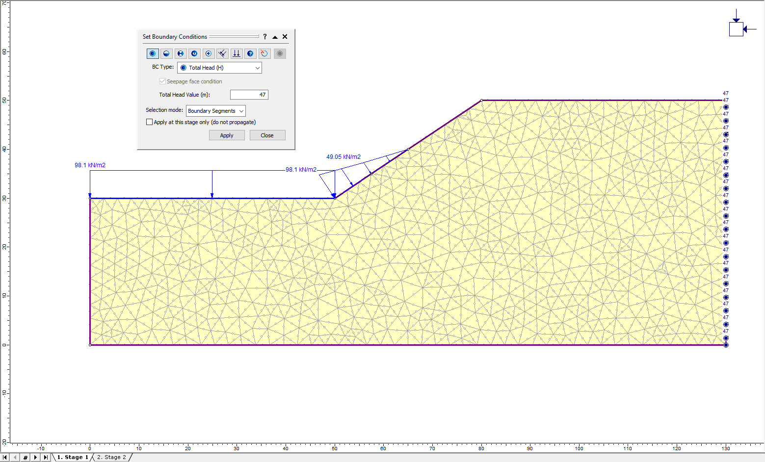
- In the dialog, change the Total Head Value to 40. Click on the left vertical boundary, the horizontal segment at the base of the slope and the bottom two segments of the slope and click apply. The model should look like this:
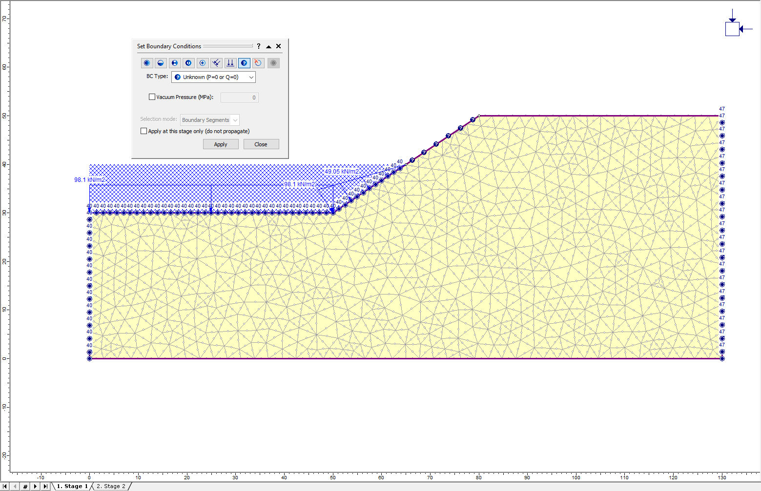
RS2 displays the ponded water based on the specified total head boundary conditions. Finally, unknown boundary conditions must be set for the rest of the slope face, it is not known where the water table will intersect the slope. - In the Set Boundary Conditions dialog, select Unknown (P=0 or Q=0) for the BC Type.
- Click the top segment of the slope face and click Apply.
- Click the Close button and the model should look like this:
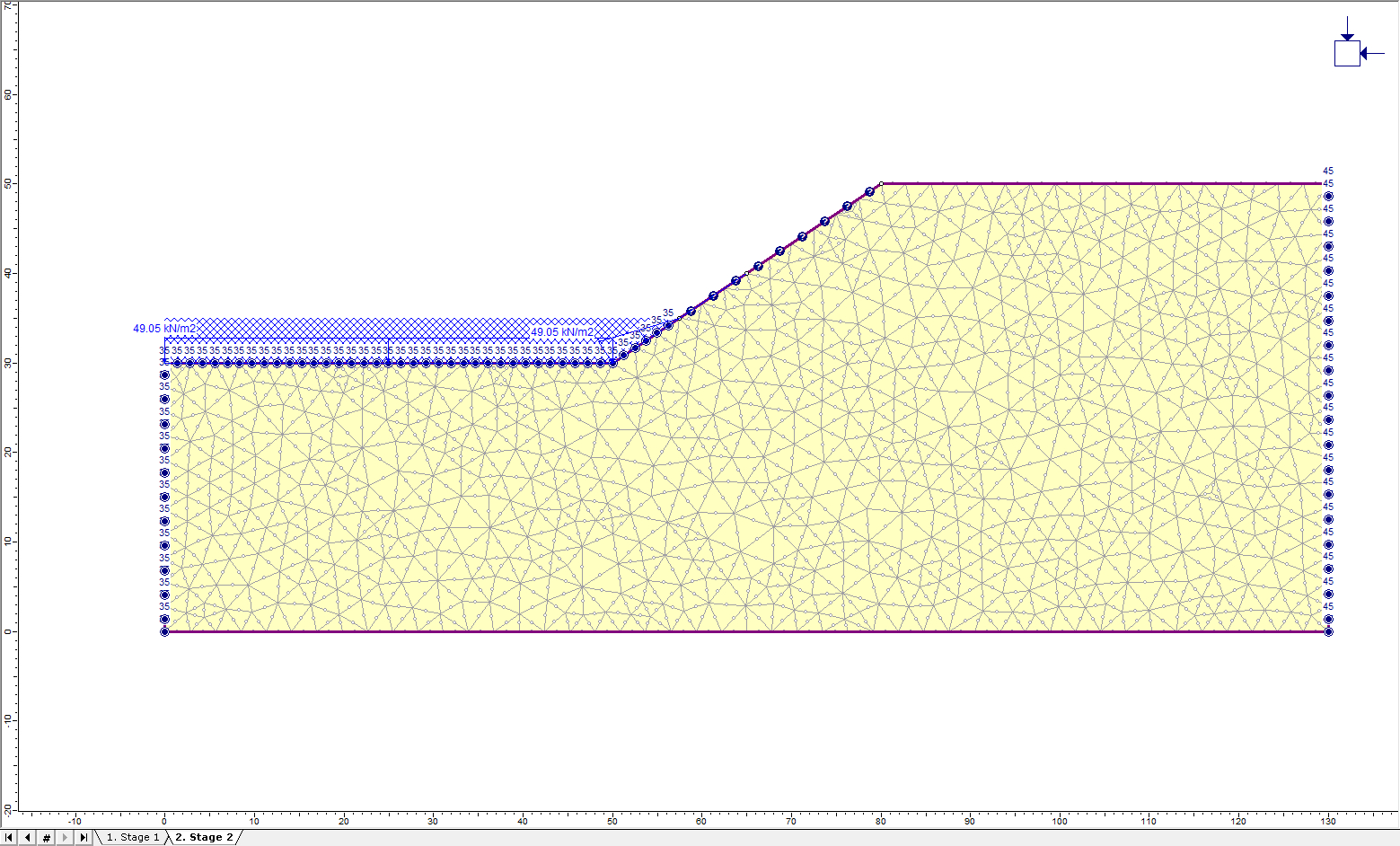
- Now click the tab for Stage 2. In Stage 2, the ponded water will be lowered.
- Select: Groundwater > Set Boundary Conditions
- Select Total Head (H) for the BC Type. Set the Total Head to 45 m. Select the right vertical boundary and click Apply.
- Set the Total Head Value to 35 m. Click on the left vertical boundary, the horizontal boundary at the base of the slope, and the bottom section of the slope face and click Apply.
- Change the BC Type to Unknown (P=0 or Q=0). Click on the section of the slope just above the water table (the middle section of the slope face) and click Apply.
- Select the Close button to close the dialog.
The model should look like this for Stage 2.
5.2 Hydraulic Material Properties
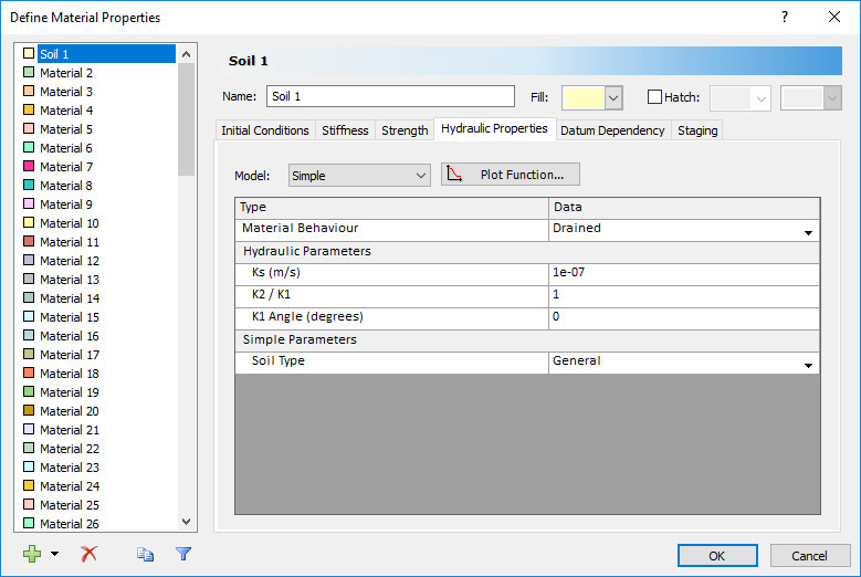
- Select: Properties > Define Hydraulic
- Select the model that dictates the permeability transition from saturated to unsaturated soil. Leave the model as the default (Simple). Leave the default value of 1e-7 m/s.
6.0 Compute: Drawdown with Finite Element Groundwater Analysis
- Select: Analysis > Compute
Because RS2 is performing a Shear Strength Reduction analysis, the model will take several minutes to run.
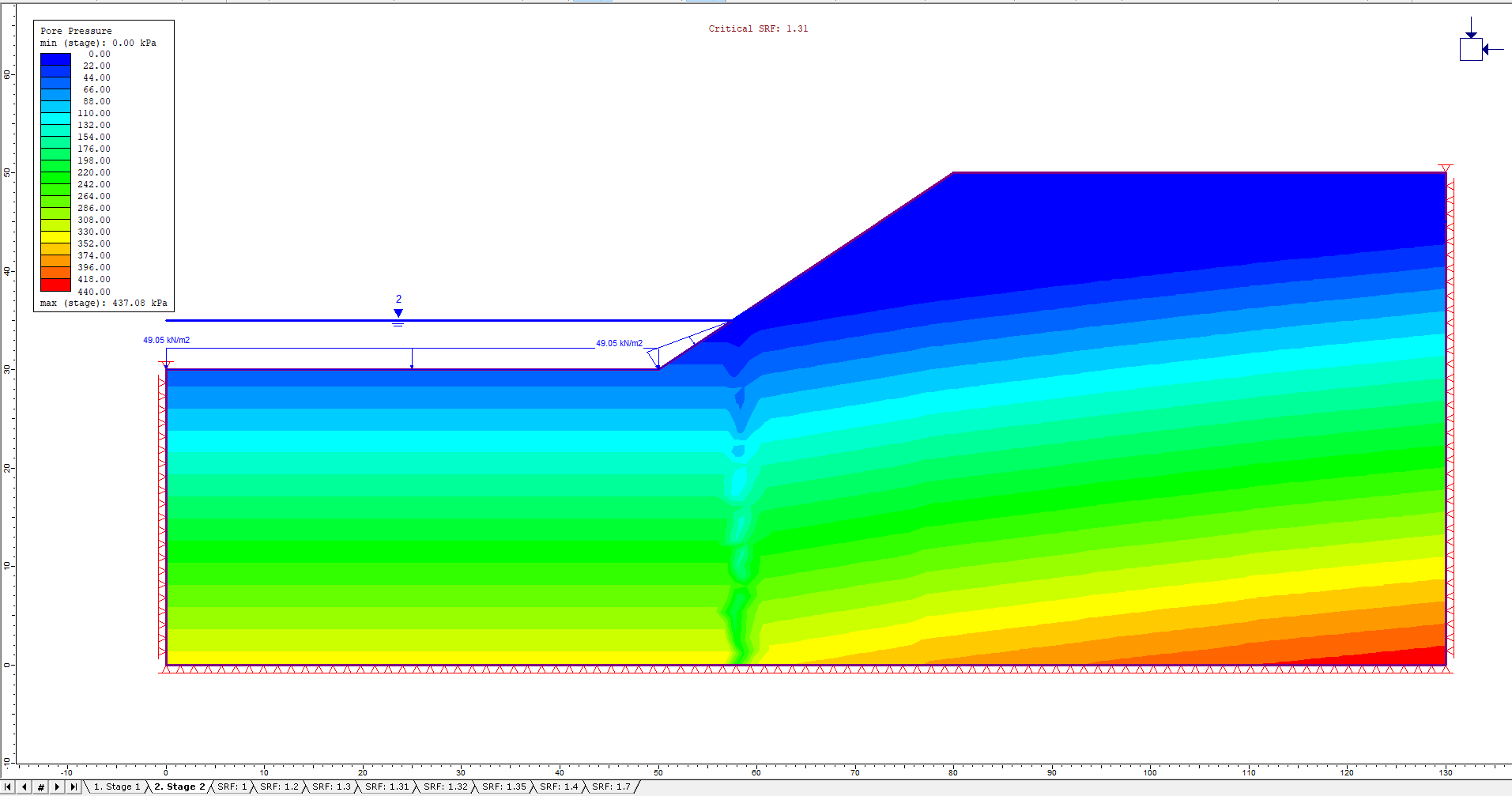
7.0 Results and Discussion: Finite Element Groundwater Analysis
- Select: Analysis > Interpret
The maximum shear strain for the critical strength reduction factor for the second stage is now shown. This is slightly lower than the SRF calculated for the model with Piezometric lines.
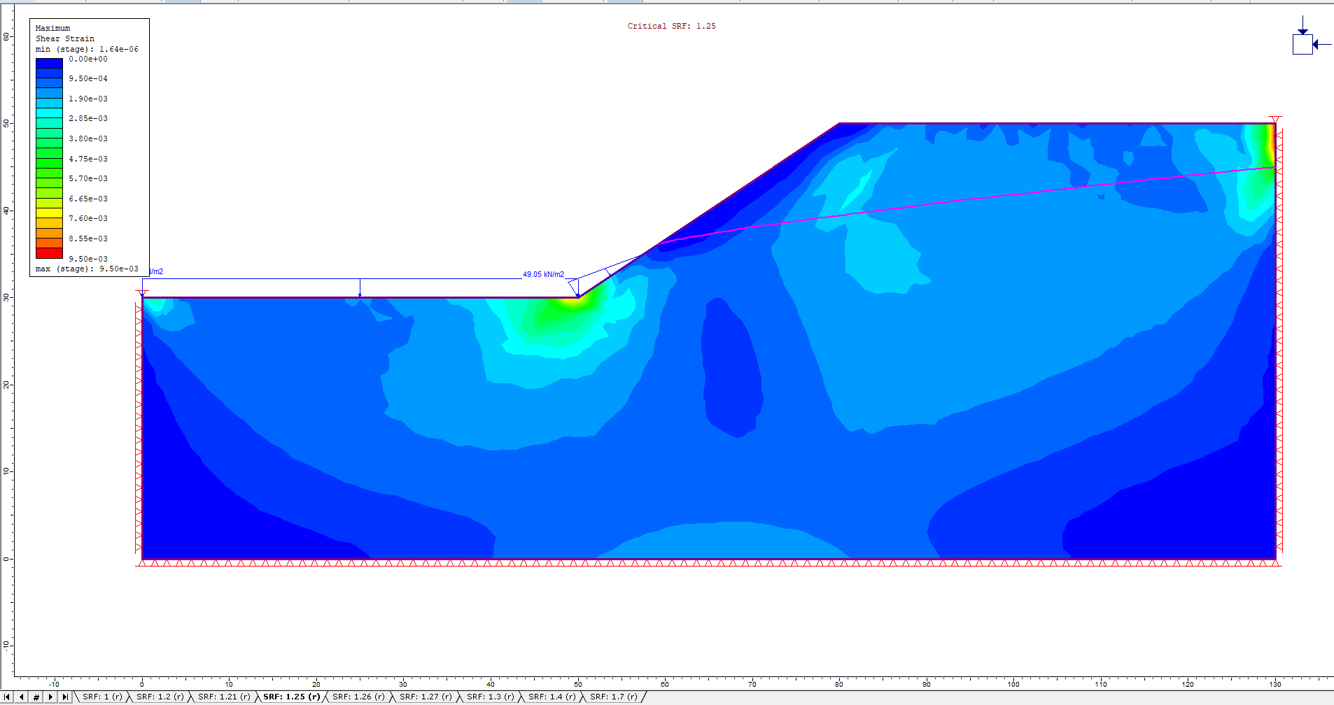
Click the tab for SRF: 1.3 to better view the critical failure surface:
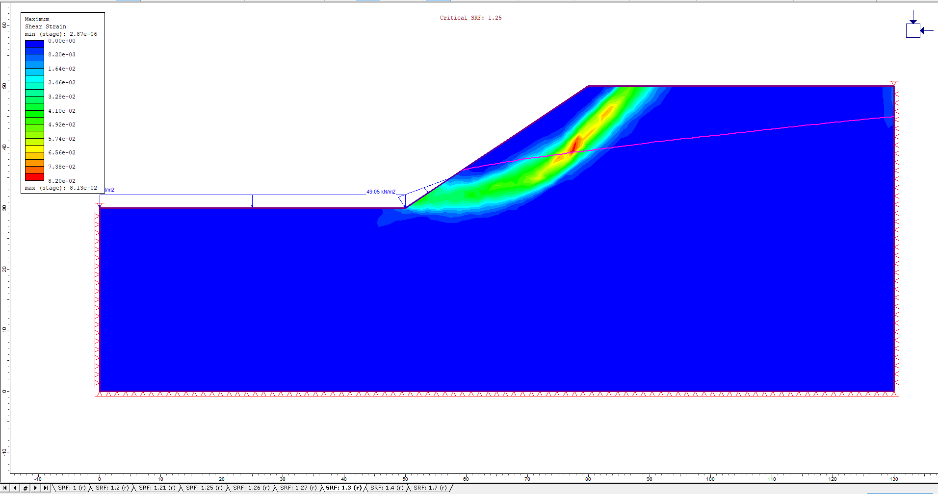
This is similar to the failure surface in the model with piezo lines.
To view stage data prior to the SSR analysis:
- Select: Data > Stage Settings
- Set the Reference Stage to Not Used, and the Visible Stage to Stage 1.
- Click OK. The maximum shear strain in Stage 1 is now visible. Change the plot to Pore Pressure using the drop-down menu in the toolbar to see the pore pressure in stage 1. Click the tab for Stage 2 to see how the pore pressure decreases as the boundary conditions change.
- View both models simultaneously by selecting Window > Tile Vertically
- Click on the window showing the pore pressures in the piezo line model. Select Stage 2. The piezo line isn’t visible because it is the same colour as the contours.
To change the piezo line colour: - Select: View > Display Options
- Under Boundaries, change the Piezometric line colour to pink as shown.
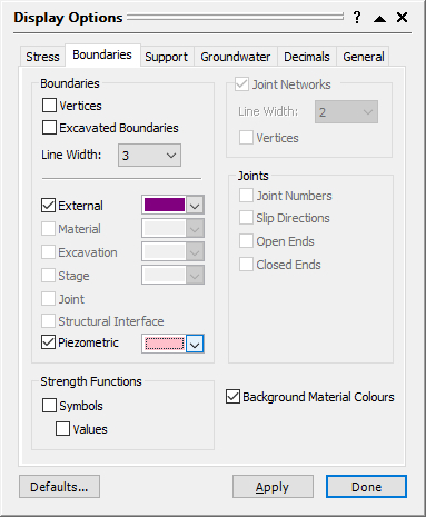
- Click Done.
To facilitate comparison between the two models, the contour range should be the same. - Select: View > Contour Options and select Custom Range.
- Set Min to -120 and Max to 480.
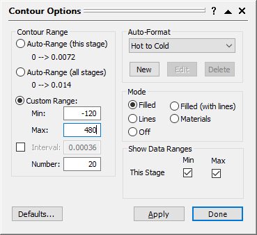
- Click Done and the screen should look like this:
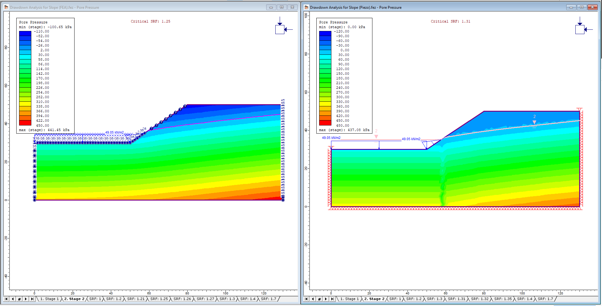
The pore pressures are essentially the same for the two models. The main difference is that the finite element groundwater model exhibits negative pore pressures (suction) above the water table.
The other difference between the models is that the contours are smoother for the finite element groundwater analysis. The results from this model are likely more accurate than the results from the model with piezo lines. The piezo line model guessed at the water table profile and the water table was then used to compute pore pressures. In the finite element groundwater model, pore pressures are calculated based on the boundary conditions, and the water table shows where the pore pressure is 0.
This concludes the Drawdown Analysis for Slope tutorial.