Dynamic Analysis of Machine Foundation
1.0 Introduction
In this tutorial, RS2 is used to simulate a foundation experiencing cyclic machine loading. This tutorial covers the basics of setting up a model for dynamic analysis in RS2 and interpreting the dynamic analysis results.
2.0 Constructing the Model
- Select: File > Recent Folders > Tutorial Folder
- Open the Dynamic Analysis of Machine Foundation (Initial) file
This file has the model geometry created, boundaries defined, meshed, and material properties defined and assigned. The tutorial begins with defining a machine load that will be applied to the foundation.
2.1 Dynamic Loads

- Select: Dynamic > Define Dynamic Load

- The Define Dynamic Loads dialog will appear, allowing dynamic loads to be defined in the X and/or Y directions. Name the load “Machine Load”. Make sure the Type field is set to Distributed Force. Check the X check box and press the Define button to define a force-time history. This will open the Function Defining Dialog
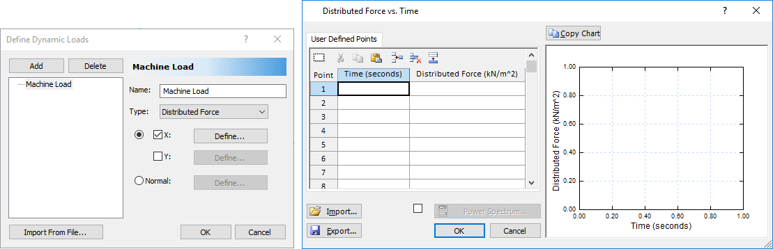
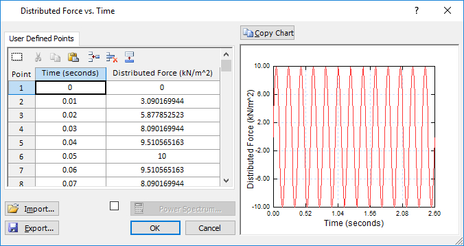
The value of the force at each time step may now be inputted in the table provided on the left side of the dialog and the resulting force history is plotted on the right side. The force that will be applied along the top of the foundation is a harmonic force with a frequency of 5 Hz and an amplitude of 10 kN/m, resulting in a total maximum force of 80 kN over the surface of the 8-meter-wide concrete foundation.
- Click the Import button in the Distributed Force vs Time dialog and select the file machine_load.txt. This will import the desired harmonic load.
- Click OK to save the force function and to close the Force vs. time dialog and click OK once more to close the Dynamic Loads dialog.
The machine load has been defined, now it must be added to the model.
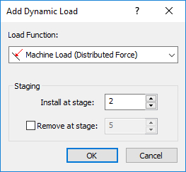
- Select: Dynamic > Add Dynamic
- Select: Load Function > Machine Load (Distributed Force) and click the OK button.
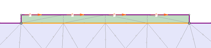
- Zoom in to the foundation and select the top line edge.
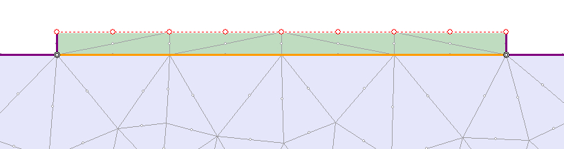
- Right-click and select Done Selection
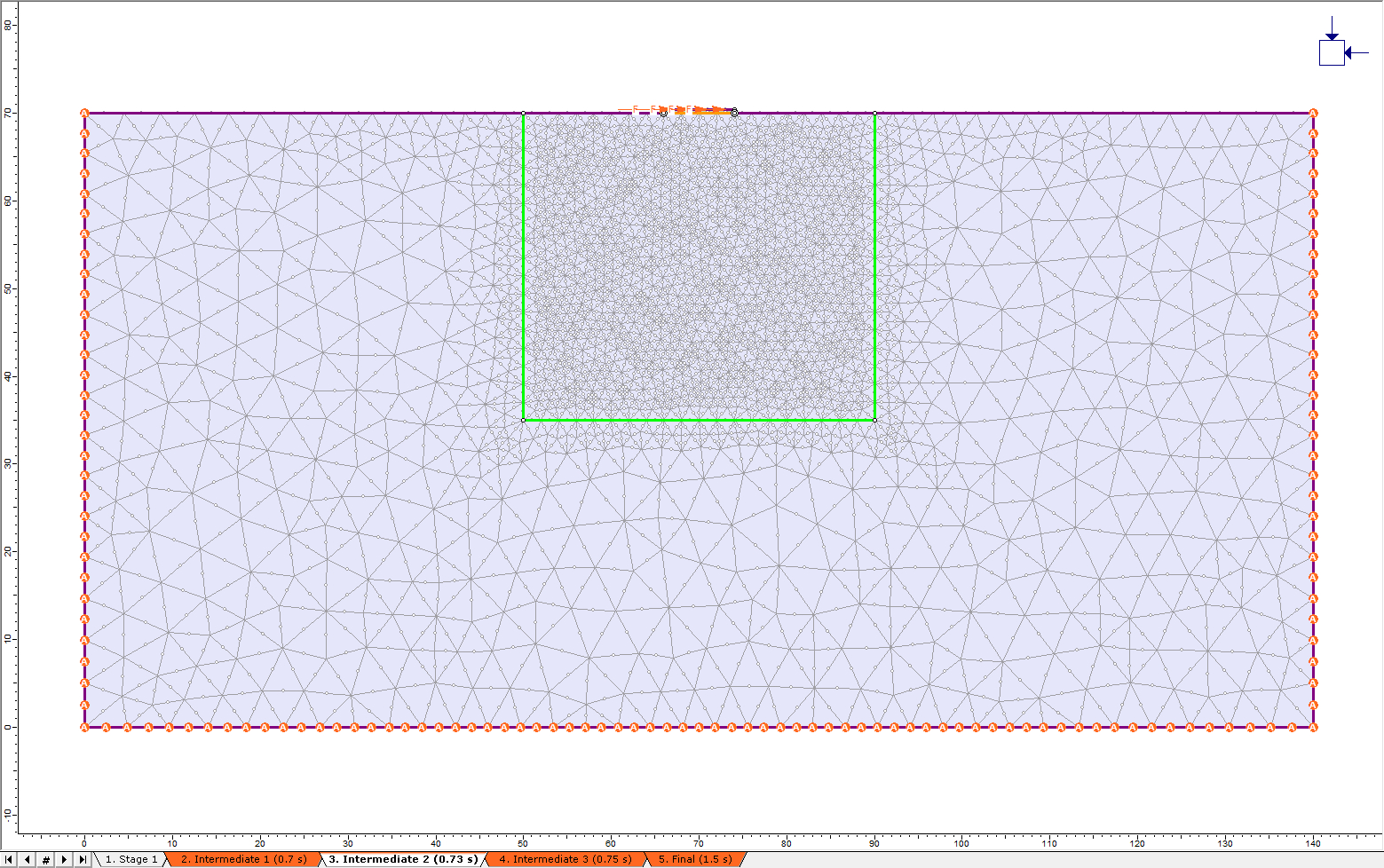
The distributed machine load has now been added to the top surface of the concrete foundation.
2.2 Dynamic Boundaries
RS2 provides several dynamic boundary conditions and elements that are utilized only in dynamic analysis. For this model absorbing boundaries will be applied on the lateral and bottom external boundaries of the model to absorb incoming shear and pressure waves travelling in the soil.
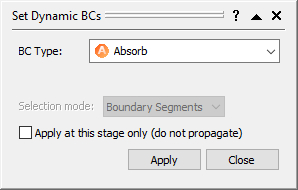
- Select: Dynamic > Set Dynamic Boundary Conditions

- Make sure that the BC Type is set to Absorb.
- Use the mouse to select the three line segments that comprise the lateral and bottom boundaries of the model. Note that absorbing boundaries may only be applied to line segments.
- Right-click and select Done Selection. Close the dialog.
The dynamic boundaries are now correctly applied. These boundaries are only visible when a dynamic stage is being viewed and the Dynamic tab is selected (in this case stages 2 to 5).
2.3 Time Query Line
Several time steps will occur between the defined stages and RS2 will not output data for all the nodes for these time steps. The modeller allows the user to specify points in the mesh, called Time Queries, where the dynamic data will be recorded for all dynamic time steps occurring in the simulation. In addition to this, a Time Query Line may be added by the user to obtain graphs that provide a visual representation of the motion of points on a line over time.
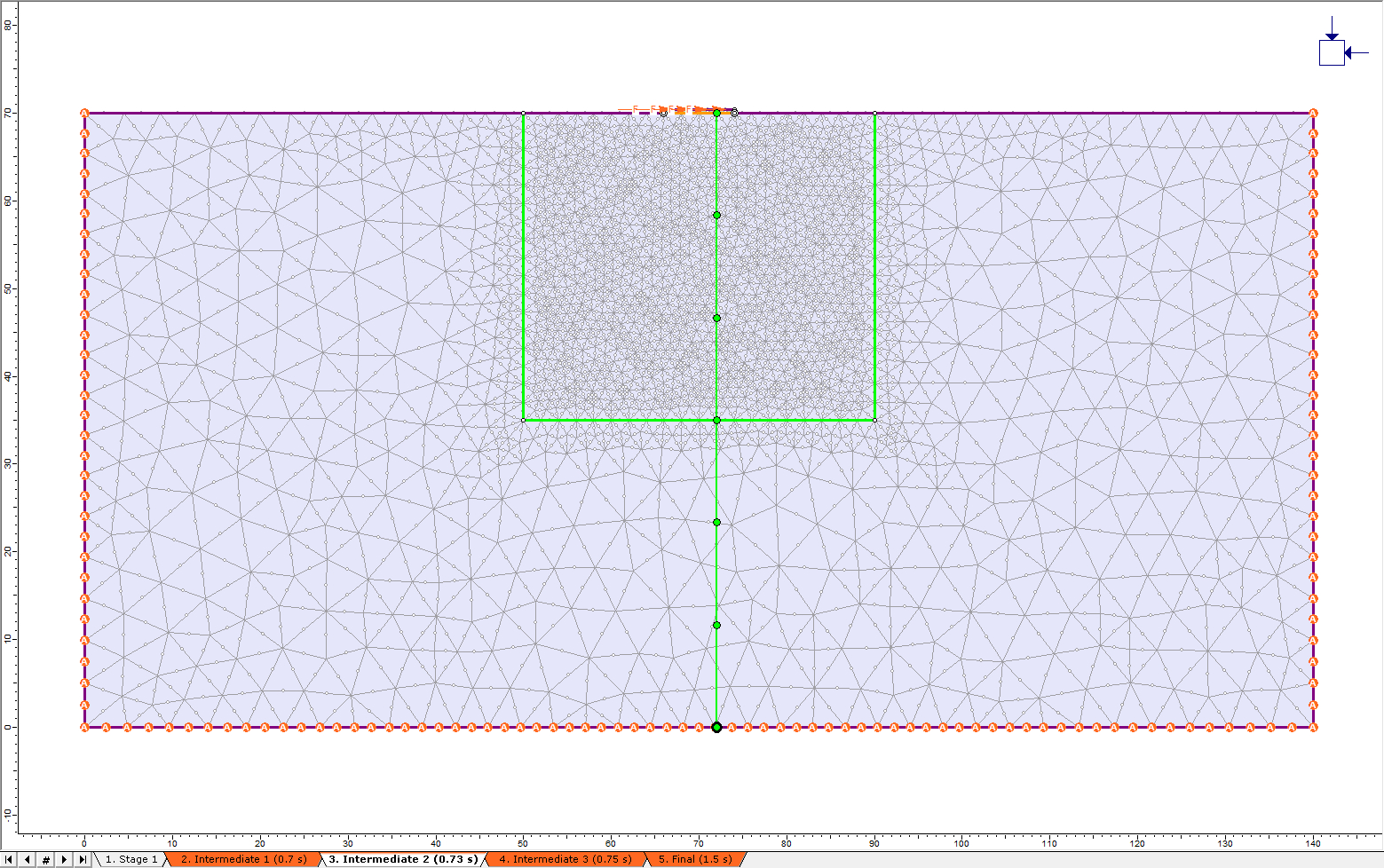
- Select: Dynamic > Time Query > Add Time Query Line

- The Specify Query Locations dialog will appear asking how many evenly spaced points should be placed on the query line. Specify 7 query points. Select OK.
- Clicking anywhere will place a vertex that the query line will contain, or the exact coordinates may be typed in. Add a time query line with the following endpoints: (72, 0), and (72,70).
- Save the model before proceeding to compute.
3.0 Compute
- Select: Analysis > Compute

The analysis should take a few minutes to run, depending on the specifications of the computer the analysis is being performed on.
4.0 Results and Discussion
- Select: Analysis > Interpret

The model is producing only values of zero for this stage because there is no external force, field stress or gravity applied at stage 1.
TIP: Change the viewing stage by selecting the Page Up / Page Down keys, or by placing the mouse cursor over the stage tabs and rotating the mouse wheel.
To obtain a contour that provides an understanding of how the waves propagate from the foundation, proceed with the following steps.
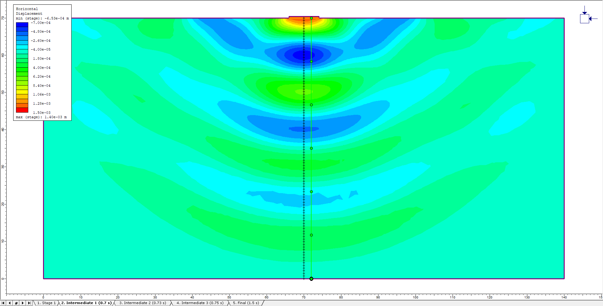
- Switch to the second stage labelled Intermediate 1.
- Select the Horizontal Displacement dataset from the Solid Displacement data option in the toolbar.
- Select: View > Display Options. Choose the Boundaries tab.
- Deselect the Material boundary option to prevent it from being displayed.
- Select Done to save and exit the dialog.
- Select: View > Contour Options. In the Contour Range section select the Auto-Range (all stages) option so that all the stages are using the same data range allowing them to be compared.
- Select Done to save and exit the dialog.
From the contour map displayed, the shear wave descending from the foundation down towards the bottom boundary is easily observed. The travelling wave is apparent from the alternating blue (cold) and green (warm) zones which represent negative and positive horizontal displacement respectively. This motion is the expected soil behaviour from a foundation with lateral machine loading acting on it.
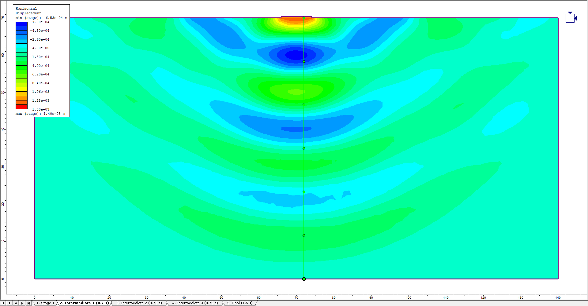
Toggling through the Intermediate stages shows the progression of the shear wave as it travels down and the formation of a new negative displacement zone at the surface as the foundation translates left.
In RS2 there are other ways to visualize this shear wave propagation. Using the Time Query Line that was added in the modeller, a visual comparison of the horizontal displacement of each of the query points can be made. The generated graph shows the amplitude reduction of the wave and the time spent travelling between the query points, which can be used as an indication of shear velocity of the soil.
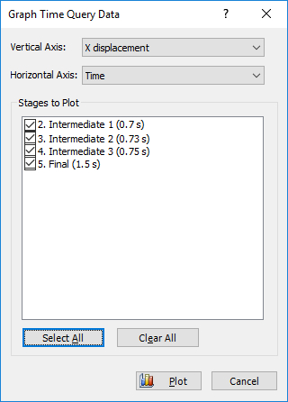
- Right-click on the Time Query Line and select Graph Time Query Line Data. The Graph Time Query Data Dialog will be open.
- Select all the dynamic stages, stages two through five. In the Vertical Axis option ensure that X displacement is selected. Select the Plot button. The time query line data is now plotted on a graph.
- Under the Chart menu, deselect Show Point Markers and select the Show Peak Values option.
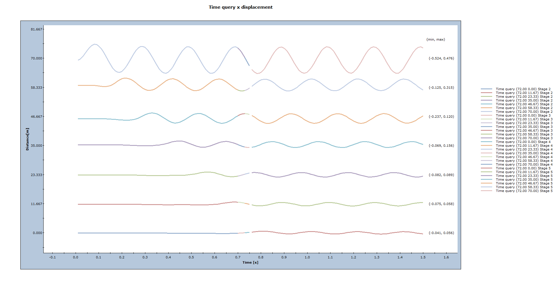
From the generated graph it is apparent that the amplitude greatly reduces from the motion at the surface to that at the bottom boundary. Comparing the time the peak values occur it is apparent that the wave takes about 0.12 s to travel from one query point to the next. The top and bottom boundaries are exceptions since they are near the surface boundary and bottom absorbing boundary.
Another graph that would be useful is that of the deformation of the soil column in the center. To obtain that shape in a graph a vertical material query line will be added at the center of the model.
- Select: Query > Add Material Query
- Enter the starting vertex of (70, 0) and another at (70, 70), right-click and select Done.
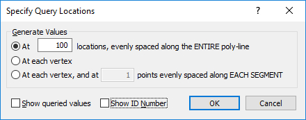
- The Specify Query Locations will open. In the first entry specify 100 locations. Turn off the Show queried values check box.
- Press OK.
Ensure that the Horizontal Displacement dataset is selected from the Solid Displacement data option. The following screen should appear:
To obtain the plot of the vertical soil profile, the following steps need to be executed:
- Right-click on the material query poly-line (not the Time Query line) and select Graph Data.
- Select only the intermediate dynamic stages to plot on the graph and click the Plot button.
- Select: Chart > Axes > Swap Horizontal and Vertical Axes Swapping to ensure that the horizontal displacement is on the horizontal axis.

A decaying sinusoidal curve centered about 0 displacement is visible. This wave is the shear wave that causes horizontal movement but travels vertically in the soil model. From the three stages displayed here, the creation of a new peak in the shear wave is evident close to the soil surface. This peak begins to propagate vertically immediately.
Additional Exercises
The interface between the foundation and soil system can be made flexible to add some realism to the system. To do this, the properties of the joint created during the tutorial will be altered.
- Select Properties > Define Joint Properties
- Change the shear stiffness to be 25 000 kPa/m and the normal stiffness to 250 000 kPa/m.
Ensure the slip criterion remains on the None option. Allowing slip in the system would allow the foundation and soil to become unattached and may cause the model to produce erroneous results.
Computing this new model and obtaining the plot from the same time query line as in the previous section shows that the displacements have increased. Where the peak displacement of the surface for the rigid joint model was 1.589 mm, the model with the elastic joint has a surface displacement of 1.801 mm.
The peaks still occur at the same times indicating that the shear wave velocity is unchanged in the soil, as would be expected since the soil's properties were unaltered.
This concludes the Dynamic Analysis of Machine Foundation Tutorial.