1 - DIPS Quick Start
1.0 Introduction
DIPS is a program designed for the interactive analysis of orientation based geological data. The program is capable of many applications and is designed for both the novice user and for the accomplished user of stereographic projection who wishes to utilize more advanced tools in the analysis of geological data.
DIPS allows the user to analyze and visualize structural data following the same techniques used in manual stereonets.
This tutorial provides a quick tour of the major plotting features of DIPS. A typical example file is used to illustrate Stereonet plots (pole, scatter, contour), rosette plots, Symbolic Plot, intersections and charting.
Topics Covered in this Tutorial:
- Grid Data view (input data spreadsheet)
- Pole Plot
- Scatter Plot
- Contour Plot
- Terzaghi Weighting (bias correction)
- Stereonet Options
- Rosette Plot
- Symbolic Pole Plot
- Intersections
- Charts
Finished Product:
The finished product of this tutorial can be found in the Tutorial 01 Quick Start.dips8 file, located in the Examples > Tutorials folder in your DIPS installation folder.
2.0 Model
If you have not already done so, run DIPS by double-clicking on the DIPS icon in your installation folder. Or from the Start menu, select Programs > Rocscience > DIPS > DIPS.
If the DIPS application window is not already maximized, maximize it now, so that the full screen is available for viewing the model.
DIPS comes with several example files installed with the program. These example files can be accessed by selecting File > Recent Folders > Examples Folder from the DIPS main menu. This tutorial will use the Example.dips8 file to demonstrate the basic plotting features of DIPS.
- Select File > Recent Folders > Example Folder
 from the menu.
 - Open the Example.dips8 file. Since we will be using the Example.dips8 file in other tutorials, save this example file with a new file name without overwriting the original file.
- Select File > Save As
 from the menu.
 - Enter the file name Tutorial 01 Quick Start and Save the file.
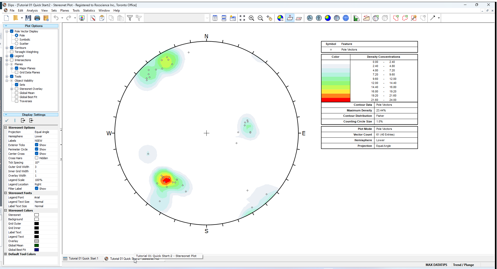
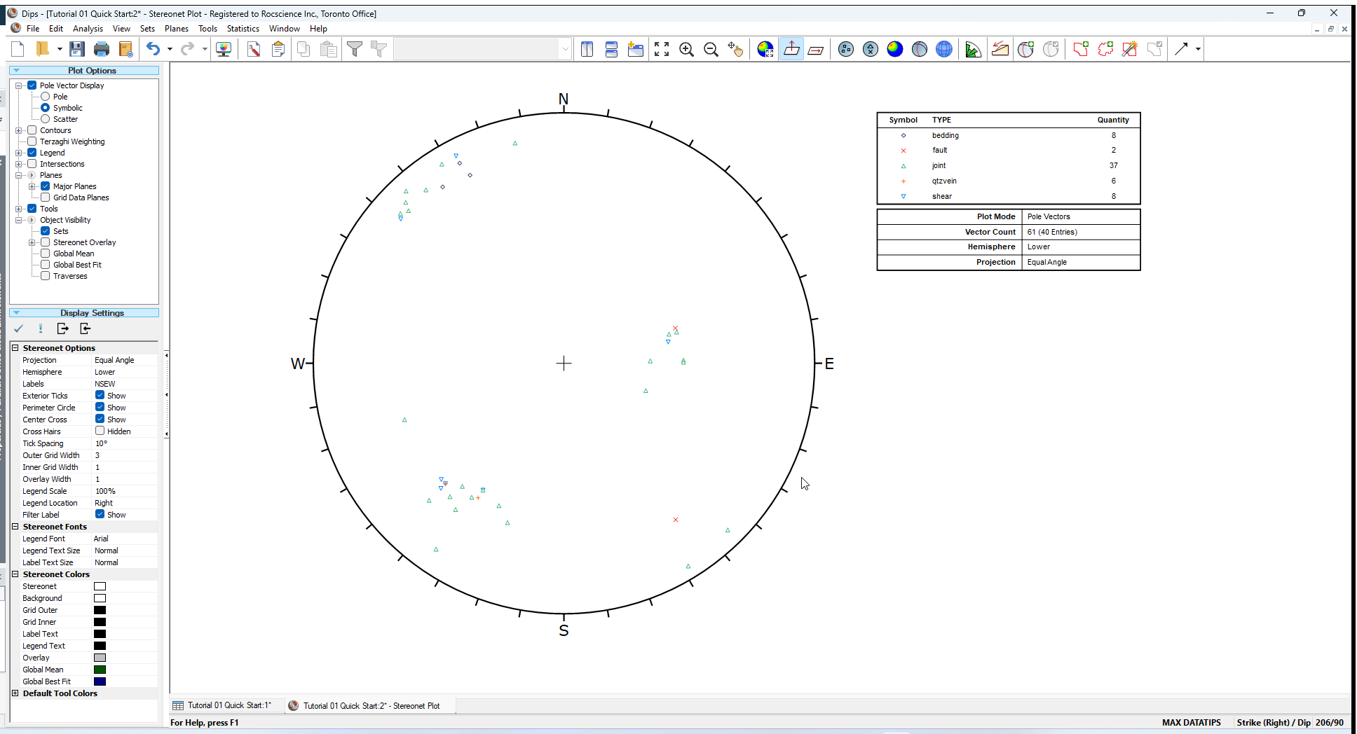
You should see the Stereonet Plot View shown in the following figure.
2.1 SIDEBAR
When you are viewing a Stereonet Plot View, the control panel at the side of the screen allows you to fully customize the data and display options for the stereonet. This control panel is referred to as the Sidebar . By selecting the check boxes and radio buttons you can overlay different types of plots (e.g., poles, contours, planes) and customize the display (e.g., colours, visibility).
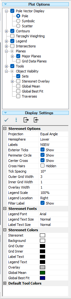
The Sidebar gives you the maximum flexibility in determining the Plot Options and Display Options. We will explore some of these options in this tutorial. For now leave the default selections in the Sidebar.
2.2 TOOLBAR SHORTCUTS
Shortcuts to commonly used plot types are available in the toolbar:
![]()
- Pole Vector Mode
 / Dip Vector Mode
- Vector Plot

- Symbolic Plot

- Contour Plot

- Major Planes Plot

- 3D Stereonet

- Rosette Plot

3.0 Grid Data view
Before we discuss the Stereonet Plot View, let’s have a look at the input data in the DIPS spreadsheet. The DIPS spreadsheet is also called the Grid Data view.
- Select the Grid Data view
 tab at the bottom of the screen.
![]()
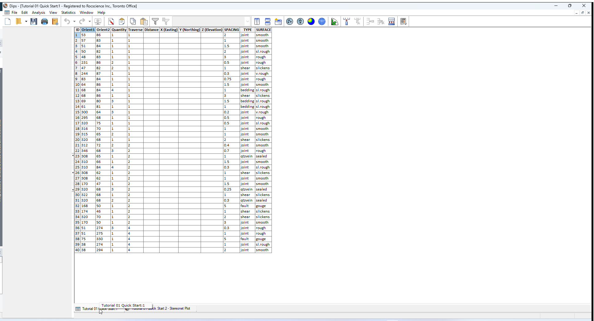
We won’t worry about the details of this file yet, except to note that it contains 40 rows, and the following columns:
- Two Orientation Columns
- A Quantity Column
- A Traverse Column
- A Distance Column
- Three X (Easting), Y (Northing), and Z (Elevation) Columns
- Three Extra Columns
In the next tutorial, we will discuss how to create the Example.dips8 file from scratch.
- Now switch back to the stereonet plot view by selecting the stereonet plot tab at the bottom of the screen.
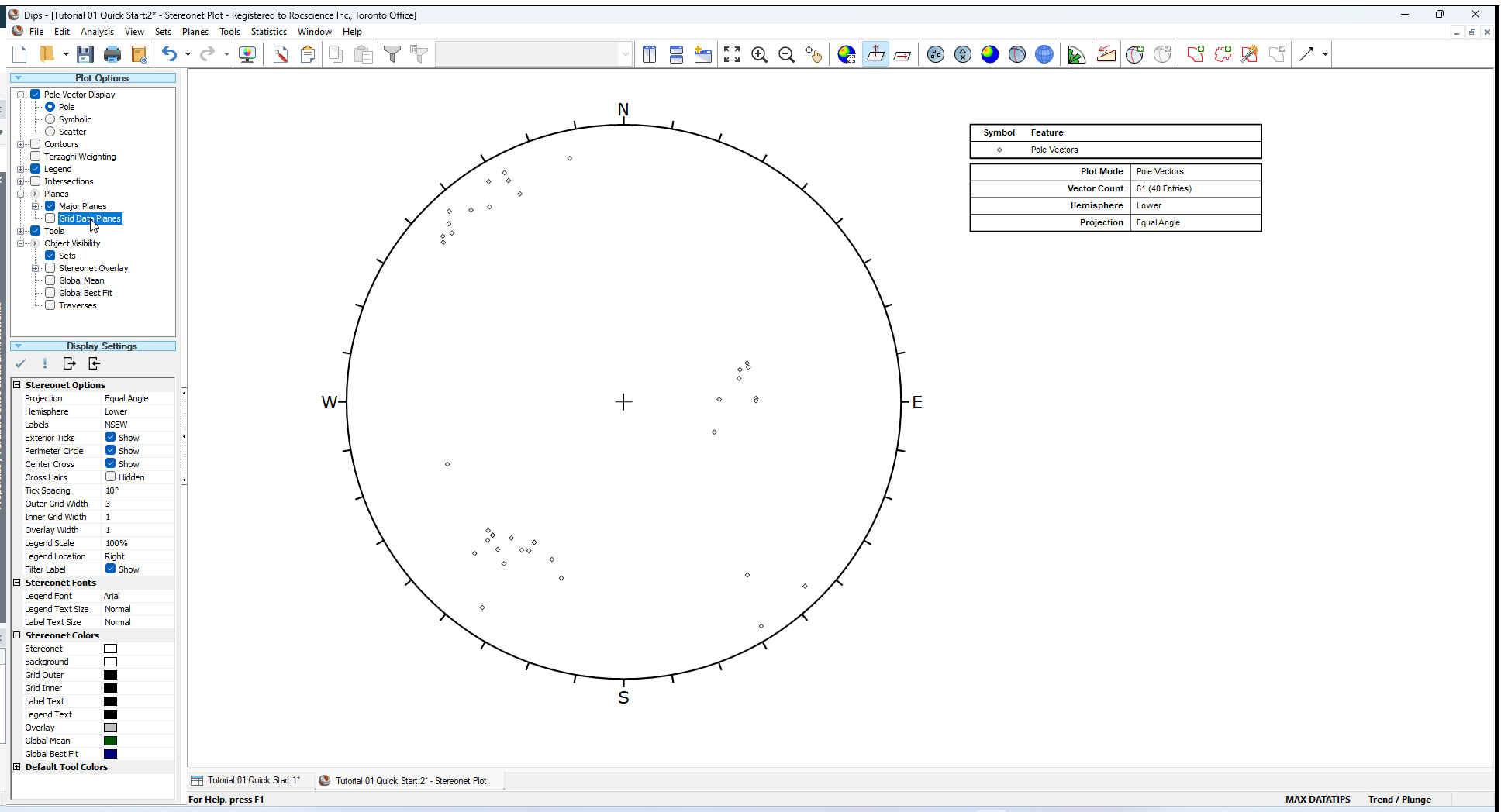
4.0 Pole Plot
The most basic representation of orientation data on a stereonet is the Pole Plot.
- Select Vector Plot option from toolbar or the View menu.
You should see the following plot.

Each pole on a Pole Plot represents an orientation data pair in the first two columns of a DIPS file.
The Pole Plot can also display feature attribute information, based on the data in any column of a DIPS file, with the Symbolic Plot option. This is covered later in this tutorial.
5.0 Dip Vector Plot
Planes can be represented as either pole vectors or dip vectors on the stereonet. A dip vector represents the maximum dip orientation of a plane and is orthogonal to the pole vector of a plane.
To view dip vectors:
- Select Dip Vector Mode option from the toolbar or the View menu.
The Stereonet Plot should look as follows.
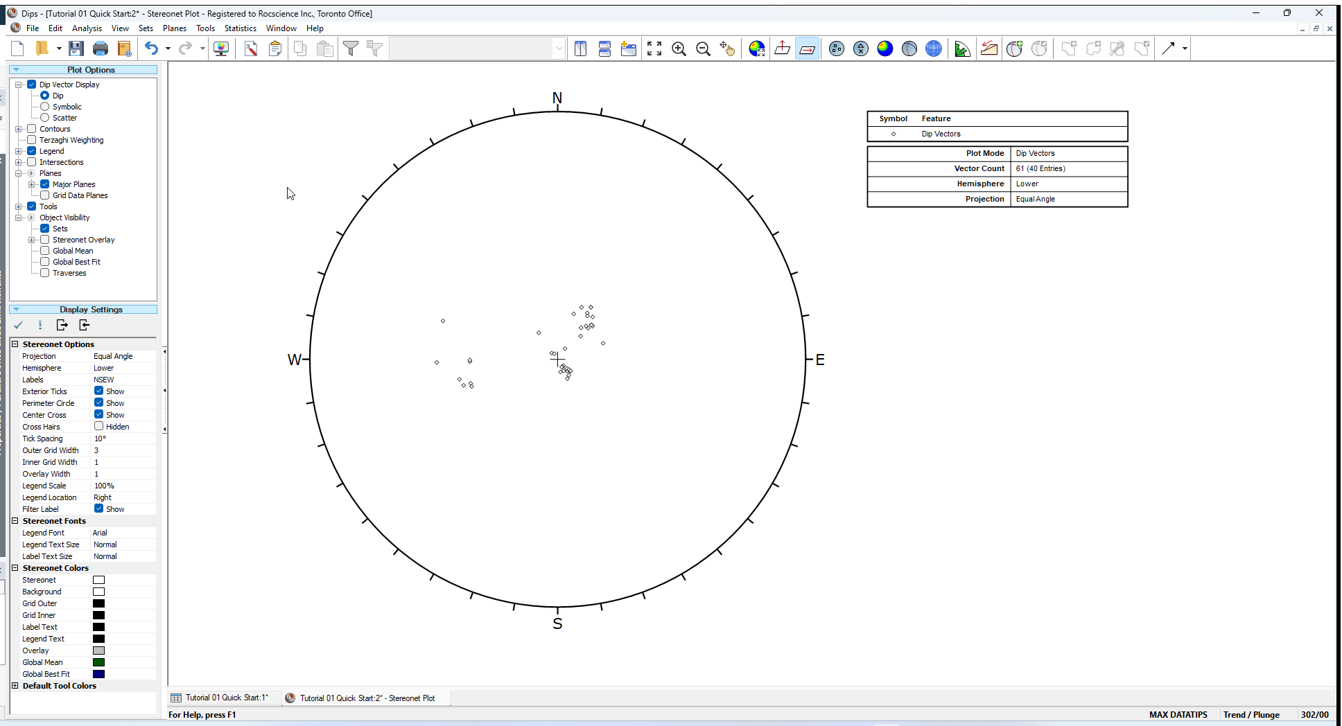
Dip Vectors are sometimes preferred for certain types of analyses, in particular Kinematic Analysis for Planar Sliding or Toppling.
In general, Pole Vectors are more commonly used and have more applications. For example, joint set orientations can only be determined from Pole Vector Plots not from Dip Vectors.
Return to the Pole Vector Plot mode:
- Select Pole Vector Mode option from the toolbar or the View menu.
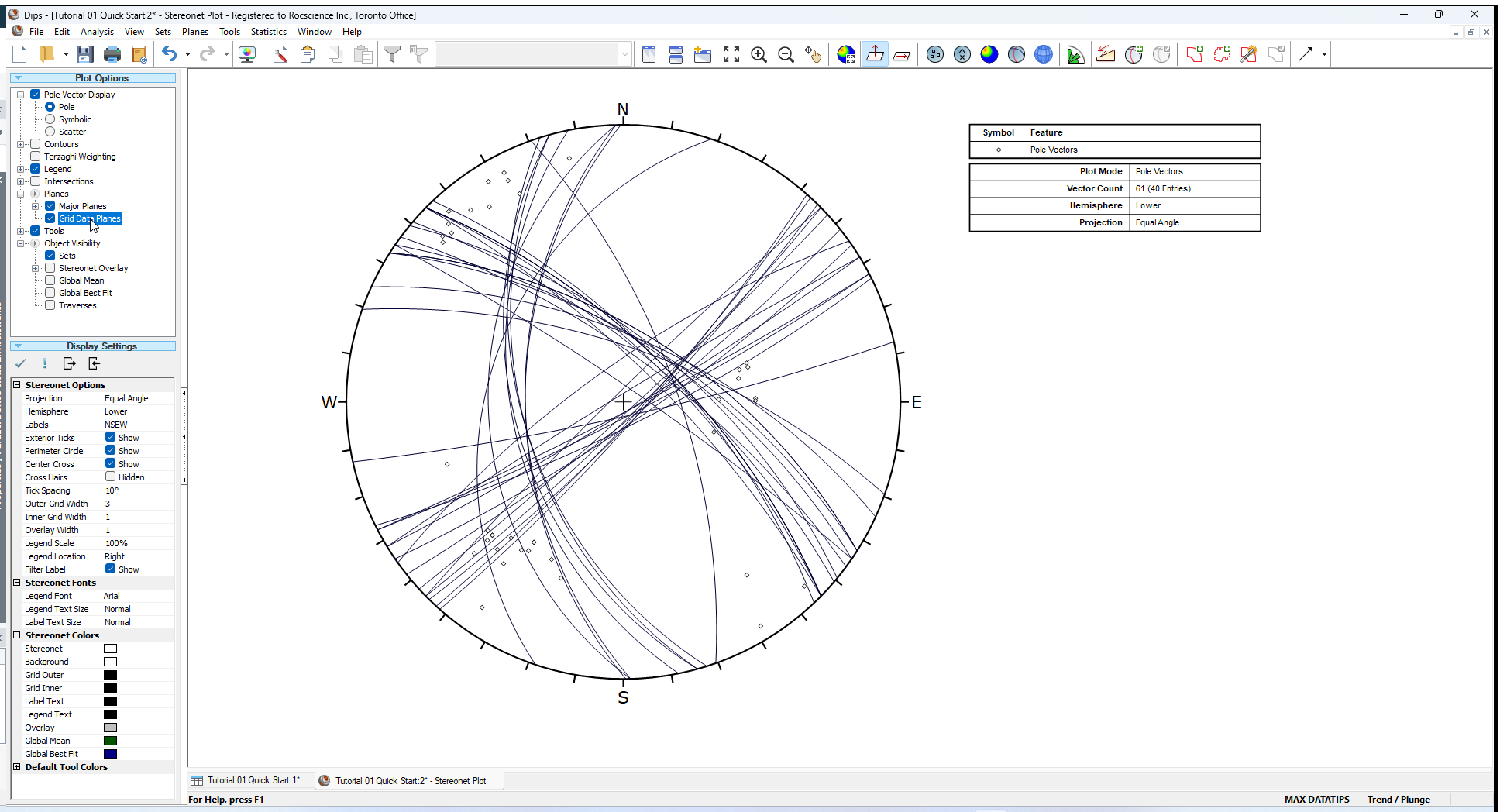
6.0 Show Grid Data Planes
To display the planes (great circles) for all of the planar data in your DIPS file:
- In the Sidebar Plot Options, select the Planes > Grid Data Planes check box
You will see all great circles displayed for all planar entries from the DIPS spreadsheet (i.e., Grid Data view) as shown below. Each great circle corresponds to a pole (or dip vector) on the vector plot.
- Turn off the display of Grid Data Planes by unselecting the Planes > Grid Data Planes checkbox in the Sidebar Plot Options.
7.0 Stereonet Legend
Note that the Legend for the Pole Plot (and all Stereonet plots in DIPS) indicates the:
- Projection Type (Equal Angle)
- Hemisphere (Lower Hemisphere)
These can be changed using Stereonet Options in the Sidebar control panel. (Equal Area and Upper Hemisphere options are available). However, for this tutorial, we will use the default projection options.
Note that the Legend also indicates Vector Count 61 (40 Entries)
- The Example.dips8 file has 40 rows, hence “40 entries”.
- The Quantity Column in this file allows you to record multiple identical data units in a single row of the file. Hence the 40 data entries actually represent 61 features, hence the total vector count of 61 poles.
8.0 Reporting Convention
As you move the cursor around the stereonet, notice that the cursor orientation coordinates are displayed in the Status Bar.
The format of these orientation coordinates can be toggled with the Reporting Convention option in the Edit menu.
- If the Convention is Trend / Plunge, the coordinates will be in Pole Vector format, and represent the cursor (pole) location directly.

- If the Convention is Dip/DipDirection or Strike/Dip (right or left hand rule for strike) the coordinates will be in Plane Vector format and represent the plane corresponding to the cursor (pole) location.


TIP: The quickest and most convenient way of toggling the Convention is to click on the box in the Status Bar to the left of the coordinate display with the LEFT mouse button.
The Reporting Convention also affects the format of certain data listings in DIPS (e.g., the Major Planes legend, the Edit Planes and Edit Sets dialogs), and the format of orientation data input for certain options (e.g., Add User Plane and Add Set Window dialogs).
9.0 Scatter Plot
While a Pole Plot illustrates orientation data, single pole symbols may actually represent several unit measurements of similar orientation.
A Scatter Plot allows you to better view the numerical distribution of measurements, since coincident pole and closely neighbouring pole measurements are grouped together with quantities plotted symbolically. The Scatter Plot Legend indicates the number of poles represented by each symbol. The size and colour of symbol indicates the approximate pole density at that location.
- Select Scatter Plot option from the View menu or the Sidebar Plot Options.
The Scatter Plot should appear as follows. 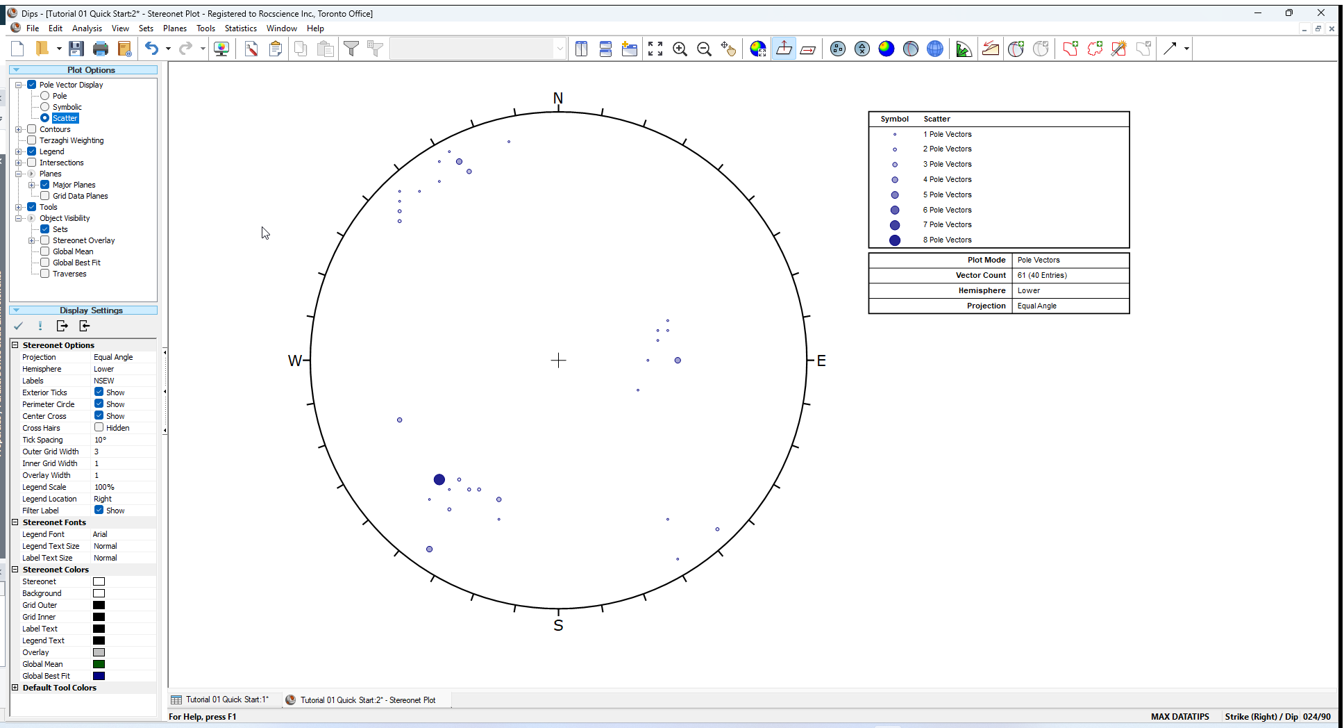
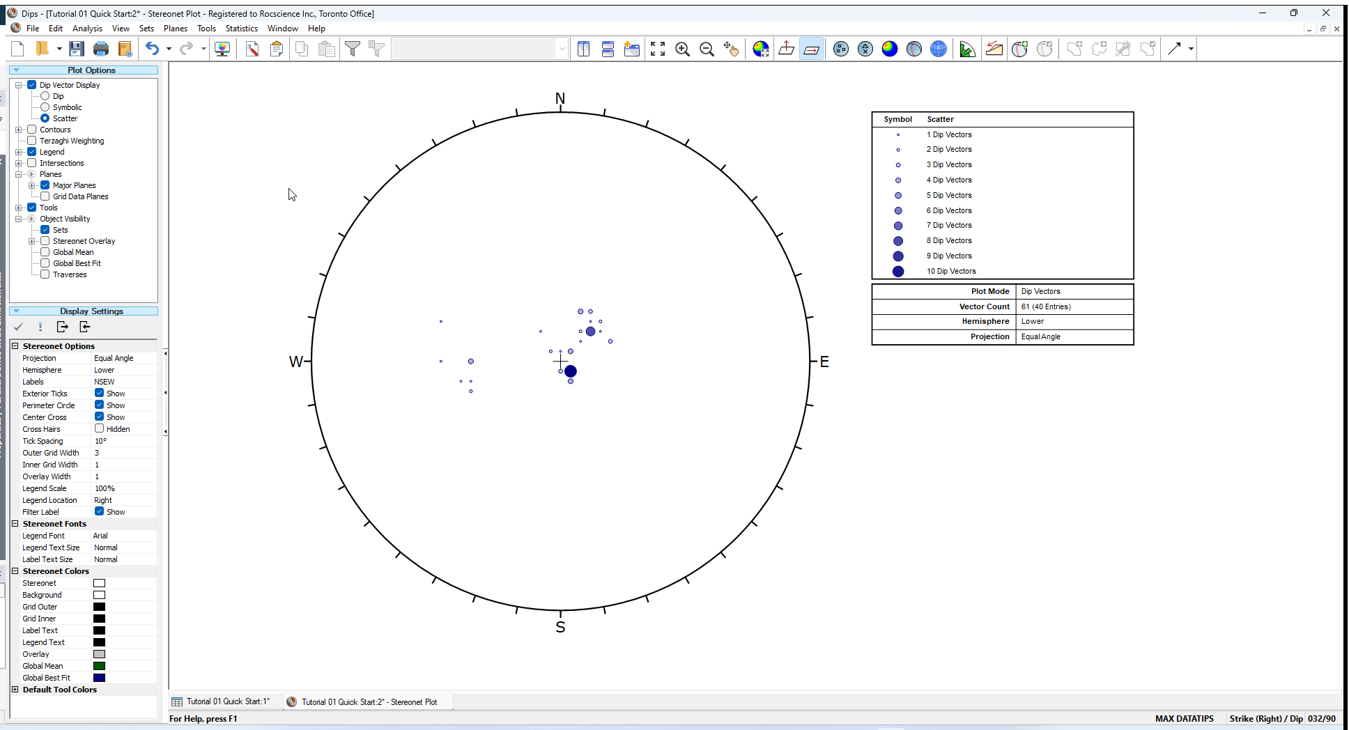
A Scatter Plot can be applied to Dip Vectors as well as poles.
- Select Dip Vector Mode from the toolbar and view the effect on the Scatter Plot.
The Scatter Plot should appear as follows.
Now switch back to Pole Vector Mode:
- Select Pole Vector Mode from the toolbar.
Let’s move on to the Contour Plot, which is the main tool for analyzing pole concentrations on a stereonet.
10.0 Contour Plot
Selecting the Contour Plot option from the toolbar or the View menu generates a Contour Plot.
- Select View > Contour Plot from the menu.
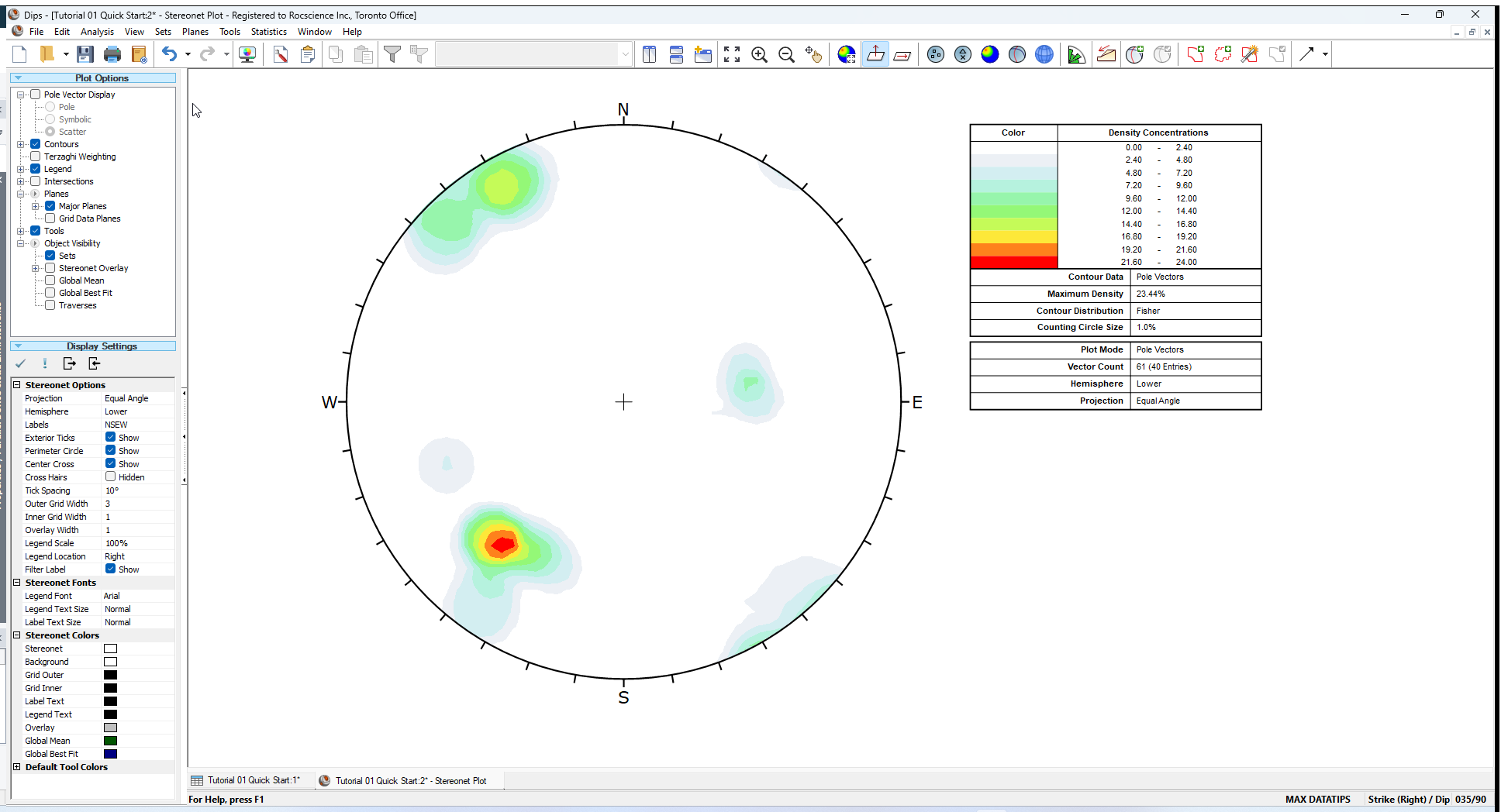
The Contour Plot clearly shows the data concentrations. It can be seen that there are three data clusters in the Example.dips8 file, including one that wraps around to the opposite side of the stereonet.
Since this file only contains 40 data entries, the data clustering in this case was apparent even on the Pole Plot. However, in larger DIPS files, which may contain hundreds or even thousands of entries, cluster recognition will not necessarily be visible on Pole Plots and Contour Plots are necessary to identify major data concentrations.
10.1 WEIGHTED CONTOUR PLOT
Since this file contains Traverse Information (Traverses are discussed in the next tutorial), a Terzaghi Weighting can be applied to Contour Plots, to correct for sampling bias introduced by data collection along Traverses.
To apply the Terzaghi Weighting to the Contour Plot:
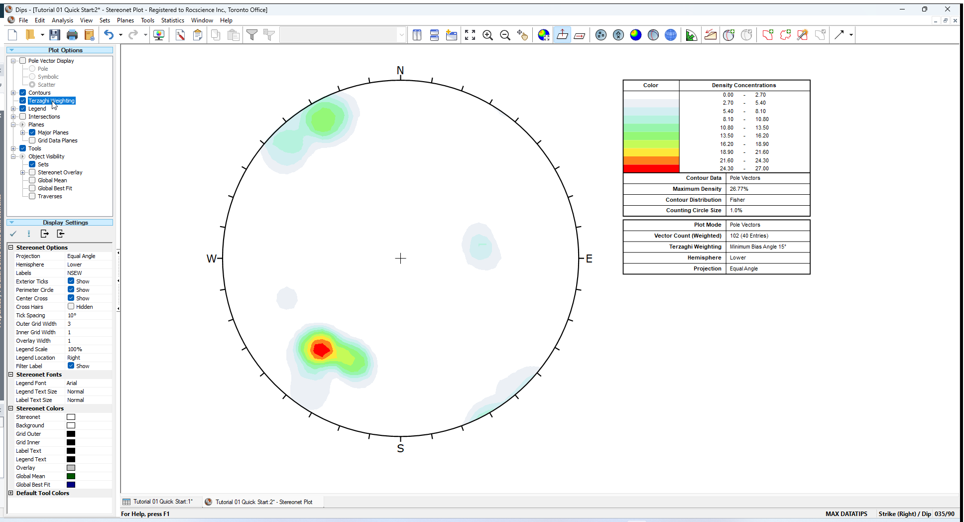
- Select the Terzaghi Weighting checkbox in the Sidebar Plot Options or View > Terzaghi Weighting from the menu.
- In the Terzaghi Weighting dialog, select the Apply Terzaghi Weighting checkbox.
Note the change in the Contour Plot. Applying the Terzaghi Weighting may reveal important data concentrations which were not apparent on the unweighted Contour Plot. The effect of applying the Terzaghi Weighting will of course be different for each file, and will depend on the data collected, and the Traverse orientations. In this case the Terzaghi Weighting does not significantly change the contour plot.
Do not use weighted contour plots for applications unless you are familiar with the limitations. For a discussion of sampling bias and the Terzaghi Weighting procedure, see the Terzaghi Weighting topic for details.
To remove the Terzaghi Weighting and restore the unweighted Contour Plot, simply de-select the Terzaghi Weighting checkbox in the Sidebar.
- Select View > Terzaghi Weighting.
- In the Terzaghi Weighting dialog, unselect the Apply Terzaghi Weighting checkbox.
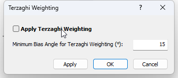
The Minimum Bias Angle for Terzaghi Weighting option allows you to set a minimum bias angle which prevents the Terzaghi Weighting factor from becoming very large. See the Terzaghi Weighting topic for details.
10.2 DIP VECTOR CONTOURS
As with pole and scatter plots, a Contour Plot can display either pole or dip vector contours, according to the setting of the Pole / Dip Vector Mode option in the toolbar.
- Select Dip Vector Mode to view the plot.
- Select Pole Vector Mode to switch back.
10.3 CONTOUR OPTIONS
Many Contour Options are available which allow you to customize the style, range and number of contour intervals. We will not explore the Contour Options in this tutorial; however, you are encouraged to experiment.
- Select View > Contour Options from the menu or right-click on a Contour Plot and select Contour Options.
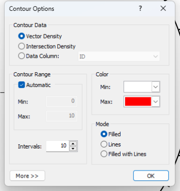
- Experiment with the various contour settings.
- Select OK to close the dialog.
See the Contour Options topic for more information.
10.4 STEREONET DISPLAY OPTIONS
In the Sidebar you will notice the stereonet Display Options.
You may choose from a variety of display options including:
- Equal Angle or Equal Area projection method
- Upper or Lower hemisphere projection
- Customized colour selections
Again, you are encouraged to experiment with these options after completing the tutorial.
11.0 Symbolic Pole Plot
We will now demonstrate how feature attribute analysis can be carried out using the Symbolic Plot and Chart options in DIPS.
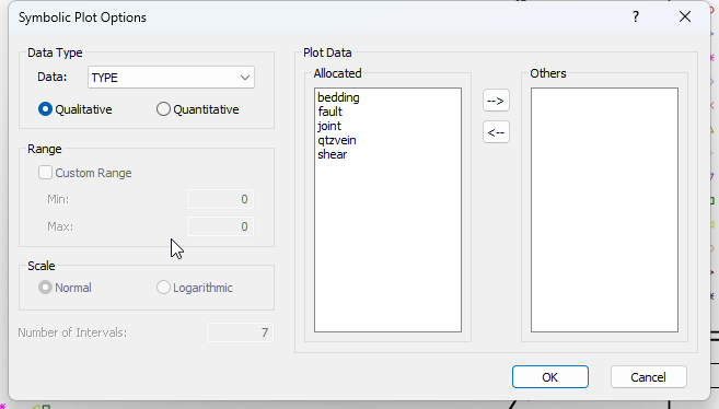
- Select Symbolic Plot option from the toolbar or the View menu.
- In the Symbolic Plot dialog, use the Data Type drop-list to select the data column you would like to plot. For example, select TYPE.
- The data in the TYPE column is Qualitative, which is the default selection so we do not have to change this. If the data were Quantitative (i.e., numeric), then we would have to select the Quantitative Data Type option.
- Notice that a list of all entries in the TYPE column appears in the Allocated list area.
- Click OK.
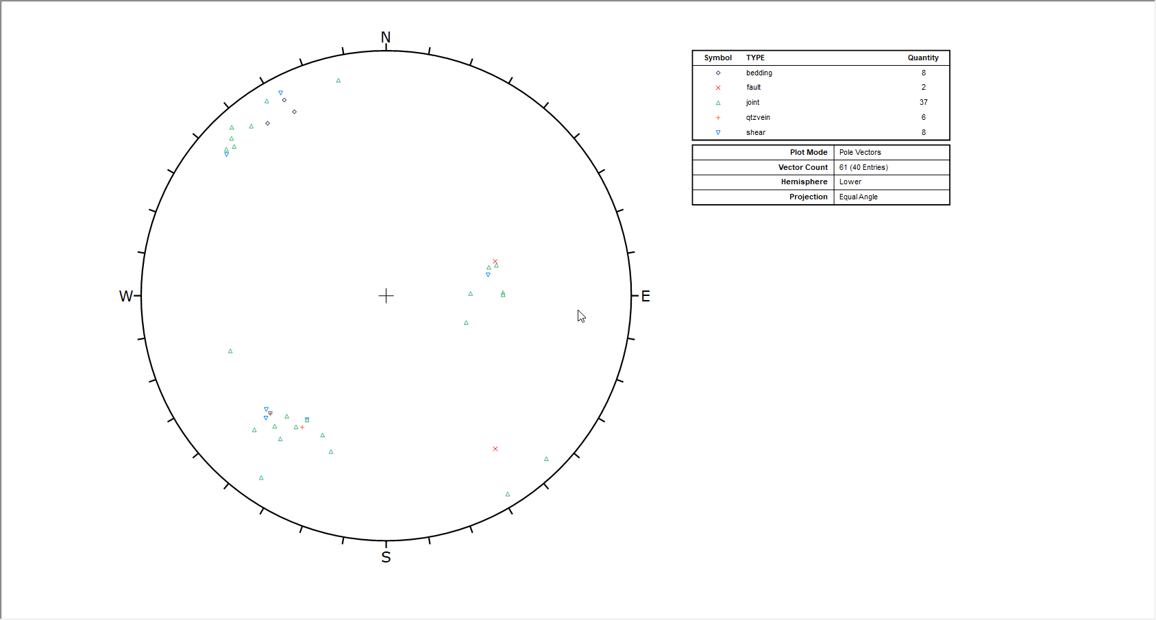
A Symbolic Plot will be generated, displaying symbols corresponding to the entries in the TYPE column as shown in the following figure.
TIP: Once a Symbolic Plot has been generated, the most recently selected properties will be “remembered” by the view. If you later switch plot types (e.g., Contour Plot, Pole Plot) you can quickly recall the current Symbolic Plot by selecting the Symbolic option in the Sidebar vector display Plot Options.
The Symbolic Plot dialog can be accessed at any time by selecting the Symbolic Plot toolbar button or the small button  beside the Symbolic option in the Sidebar or in the right-click menu.
11.1 SYMBOLIC PLOT LEGEND
In the Symbolic Plot Legend, you will notice the Quantity of each feature being plotted. This refers to the total number of poles with that label (i.e. it accounts for the Quantity Column values). If you add the Quantity numbers in the Legend, you will find that the total is equal to the Vector Count (number of Poles) listed at the bottom of the Legend, in this case, 61.
11.2 SYMBOLIC DIP VECTOR PLOT
As with pole, scatter and contour plots, the Symbolic Plot can display either poles or dip vectors, according to the setting of the Pole / Dip Vector Mode option.
- Select Dip Vector Mode in the toolbar or View menu to view the plot.
- Switch back to Pole Vector Mode in the toolbar or View menu.
11.3 CREATING A CHART FROM A SYMBOLIC PLOT
Now let’s create a corresponding Histogram, based on our Symbolic Pole Plot.
- Right-click on the Symbolic Plot. From the popup menu, select Symbolic > Create Corresponding Chart.
- In the Chart dialog, under Data to Plot, Data = TYPE is already pre-selected.
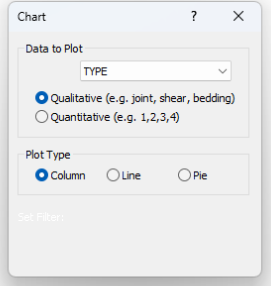
- Select OK.
A new chart view will automatically be generated, using the same data and settings selected for the Symbolic Plot.
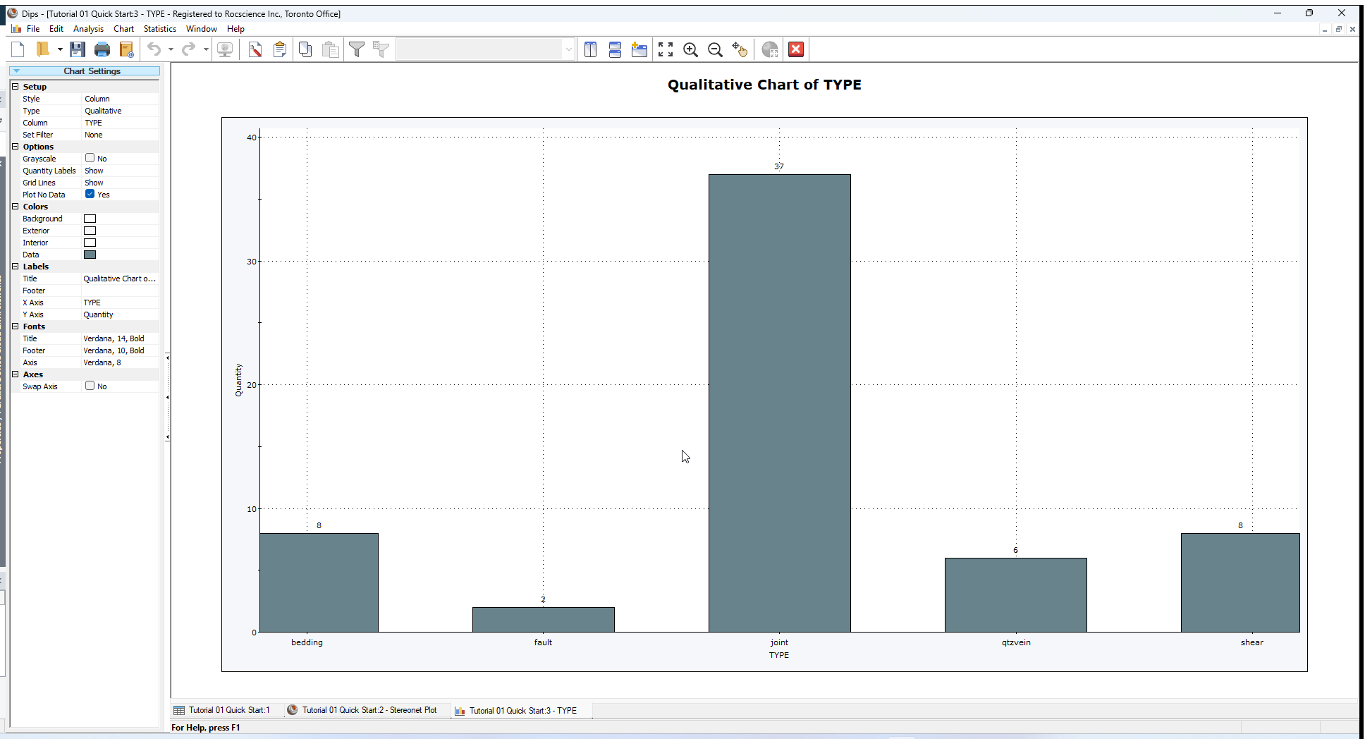
The Chart can then be customized if desired using the various Chart Settings available in the Sidebar (e.g., the Histogram can be converted to a Pie Chart or a Line graph).
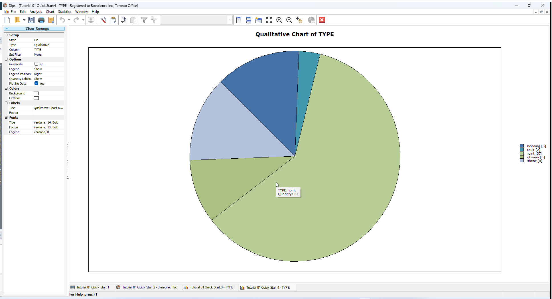
Let's look at the Qualitative Chart in Pie Style.
- Select Style = Pie in the Sidebar Chart Settings.
You should see the following chart.
Charts can also be generated directly using the Chart option  in the toolbar or the Analysis menu. The above procedure is simply a shortcut for generating a chart from an existing Symbolic Plot.
- Switch back to the Stereonet Plot View using the tabs at the bottom of the screen.
12.0 Plotting Intersections
The intersection of two planes forms a line in 3-dimensional space which can be plotted as a point on the stereonet. Planar intersections are used in kinematic stability analysis for Wedge Sliding and Direct Toppling failure modes.
Several options are available for plotting intersections.
In the Sidebar Plot Options:
- Select the Intersections checkbox. The default option is Grid Data Planes. This will plot the intersections of all planes in your DIPS file.
- Unselect the Pole Vector Display checkbox to turn off the display of pole vectors.
- Select the Contours > Intersection option to contour the intersection points.
Your screen should look as follows.
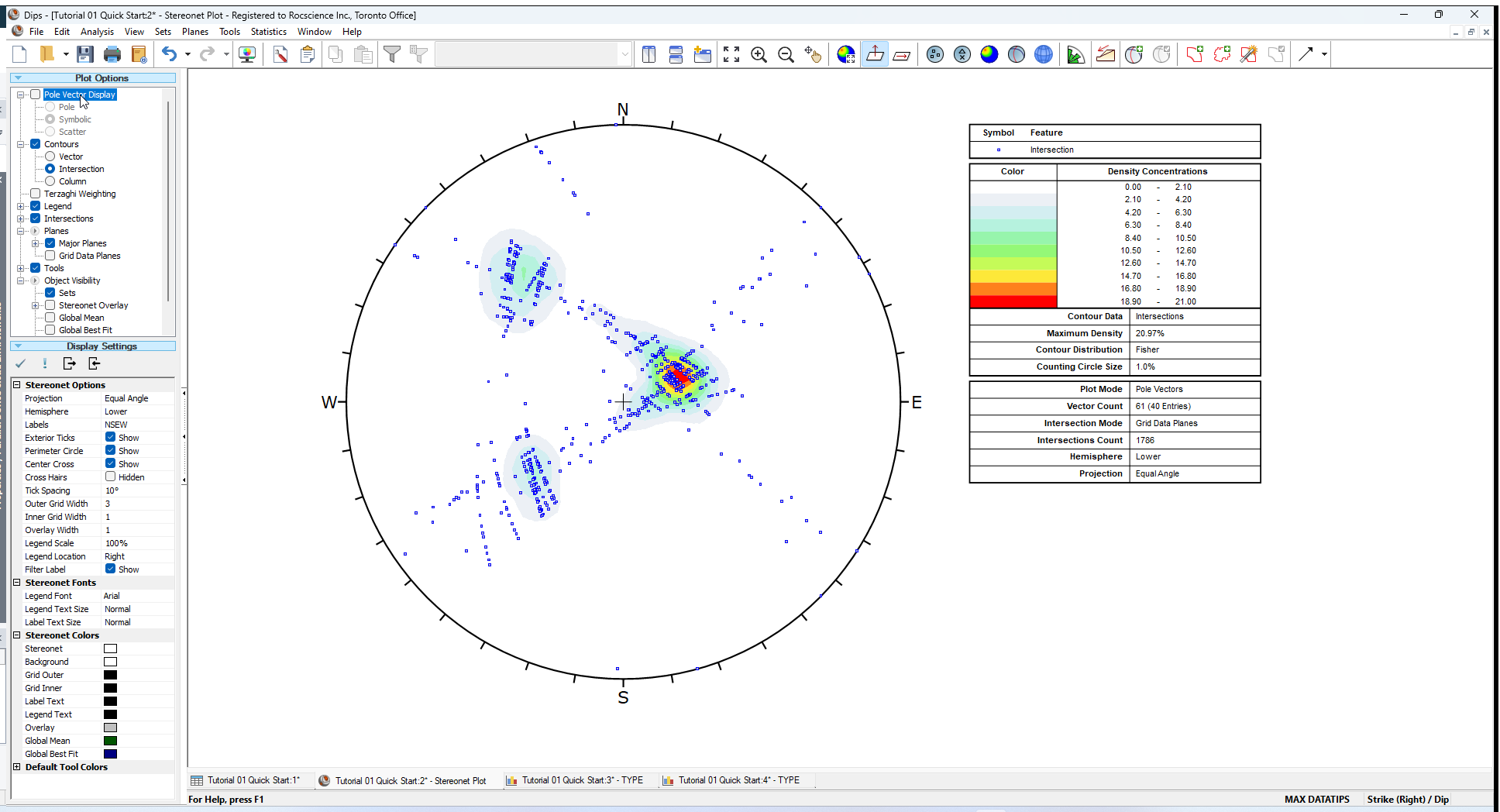
Note that the Legend indicates that Grid Data Planes Intersection Mode is being plotted and the Intersections Count.
Other intersection plotting options allow you to intersect:
- All Set Planes
- Set vs Set Planes
- User and Mean Set Planes
- User Planes
- Mean Set Planes
See the Intersections topic for further information.
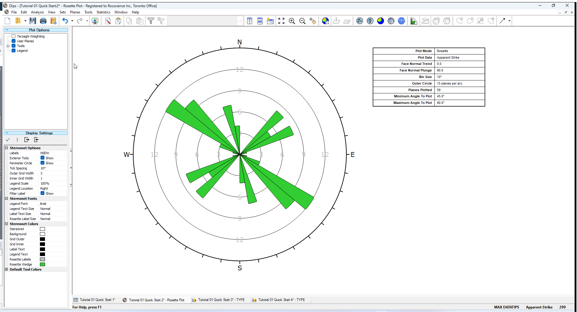
13.0 Rosette Plot
Another widely used technique for representing orientations is the Rosette Plot.
The conventional Rosette Plot begins with a horizontal plane (represented by the equatorial (outer) circle of the plot). A radial histogram (with arc segments instead of bars) is overlain on this circle, indicating the density of planes intersecting this horizontal surface. The radial orientation limits (azimuth) of the arc segments correspond to the range of Strike of the plane or group of planes being represented by the segment. In other words, the rosette diagram is a radial histogram of strike density or frequency.
To generate a Rosette Plot:
- Select Rosette Plot option from the toolbar or the View menu.
- Right-click on the Rosette Plot. From the popup menu, select Rosette Options.
- In the Rosette Options dialog:
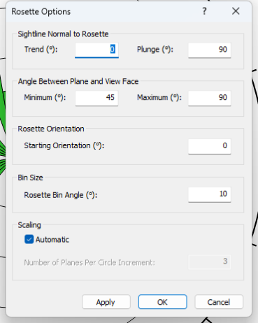
- Experiment with the various options. See the Rosette Plot and Rosette Options topics for information about the Rosette Plot Options.
- Select OK to close the dialog.
13.2 ROSETTE APPLICATIONS
The Rosette Plot conveys less information than a full stereonet since one dimension is removed from the diagram. In cases where the planes being considered form essentially two dimensional geometry (prismatic wedges, for example) the third dimension may often overcomplicate the problem. A horizontal rosette diagram may, for example, assist in blast hole design for a vertical bench where vertical joint sets impact on fragmentation. A vertical rosette oriented perpendicular to the axis of a long topsill or tunnel may simplify wedge support design where the structure parallels the excavation. A vertical rosette which cuts a section through a slope under investigation can be used to perform quick sliding or toppling analysis where the structure strikes parallel to the slope face.
From a visualization point of view and for conveying structural data to individuals unfamiliar with stereographic projection, rosettes may be more appropriate when the structural nature of the rock is simple enough to warrant 2D treatment.
13.3 WEIGHTED ROSETTE PLOT
The Terzaghi Weighting option can be applied to Rosette Plots as well as Contour Plots, to account for sampling bias introduced by data collection along Traverses.
- If the Terzaghi Weighting is NOT applied, the scale of the Rosette Plot corresponds to the actual “number of planes” in each bin.
- If the Terzaghi Weighting IS applied, the scale of the Rosette Plot corresponds to the WEIGHTED number of planes in each bin.
14.0 Info Viewer
The Info Viewer presents a formatted summary of your DIPS file input data and analysis results.
- Select Analysis > Info Viewer
 from the menu.
 - Scroll down to view the information presented in the Info Viewer.
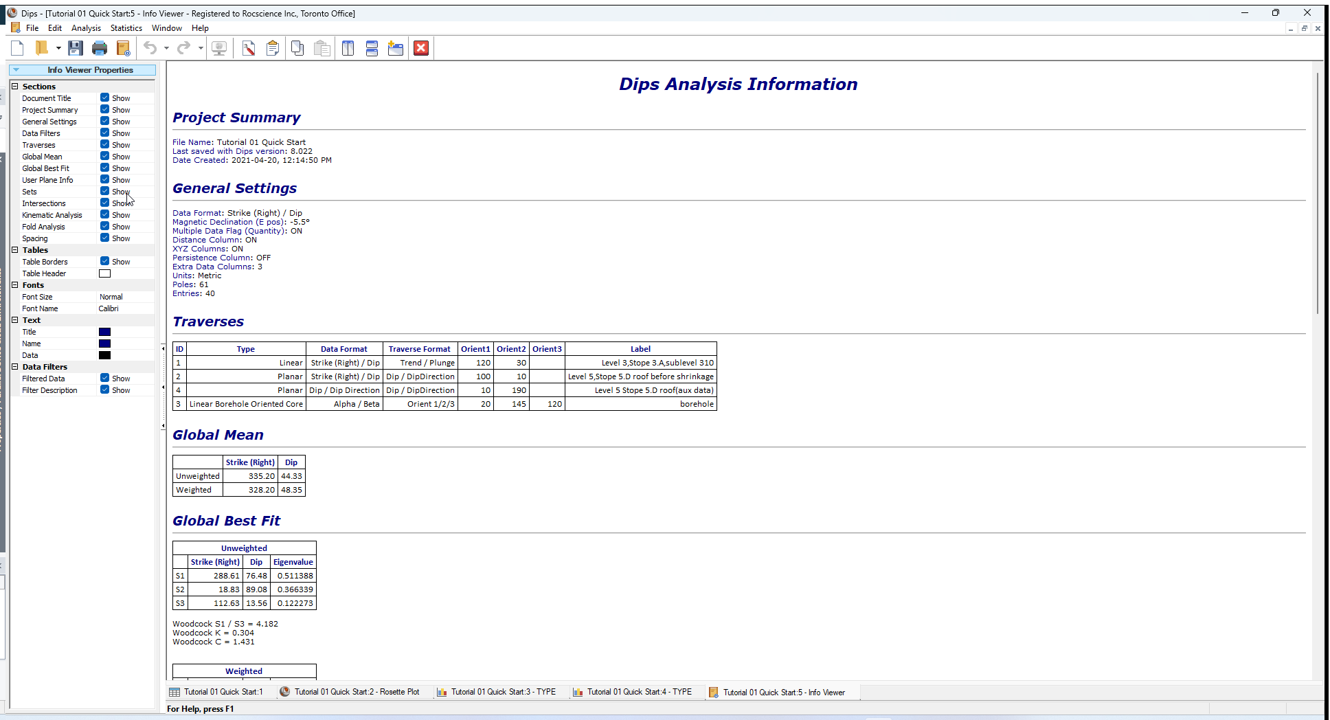
The Sidebar allows you to customize the information shown in the Info Viewer as well as the appearance (fonts, colours, etc.).
The Info Viewer information can be copied to the clipboard ( Copy  ) or saved to a file (right-click and Save As HTML) for including in reports.
When Sets are defined, all Set Statistics can be found listed in the Info Viewer. Sets are covered in Tutorial 03 - Sets (Set Window), Tutorial 04 - Sets (Set Window Freehand), and Tutorial 05 - Sets (Sets from Cluster Analysis).
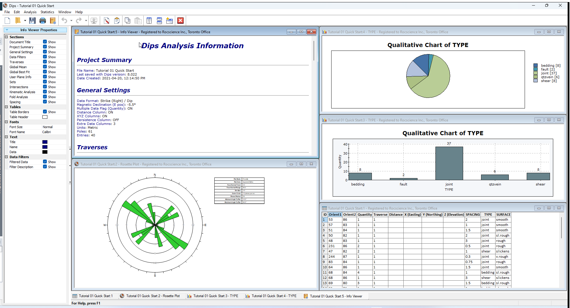
15.0 Working with Multiple Views
Now tile the views.
- Select Tile Vertically
 option from the Window menu.
 - Notice that as you click the mouse in each view the Sidebar options are updated for the focused view.
New Stereonet Plot Views can be generated at any time, by selecting the New Pole Vector Plot option in the Window menu. - Select New Pole Vector Plot
 option in the Window menu.
If all views are still open your screen may look similar to the following figure.
Display and visibility options can be customized independently for each open view. This is left as an optional exercise to explore.
This concludes the tutorial. You are now ready for the next tutorial, Tutorial 02 - Creating a DIPS File.