11 - Oriented Core & Rock Mass Classification
1.0 Introduction
Oriented core data can be processed by DIPS into true dip and dip direction, using the oriented core Traverse option. This tutorial discusses a DIPS file which uses oriented core input data. Using the additional information in the Extra Columns of the DIPS file, a rock tunneling quality index Q is estimated.
Topics Covered in this Tutorial:
- Linear BH Oriented Core Traverse
- Rock Tunneling Quality Index Q
- RQD (Rock Quality Designation)
- Estimation of JR and JA
- Tunneling Support Guidelines
Finished Product:
The finished product of this tutorial can be found in the Tutorial 11 Oriented Core and Mass Rock Classification.dips8 file, located in the Examples > Tutorials folder in your DIPS installation folder.
2.0 Model
If you have not already done so, run DIPS by double-clicking on the DIPS icon in your installation folder. Or from the Start menu, select Programs > Rocscience > DIPS > DIPS.
If the DIPS application window is not already maximized, maximize it now, so that the full screen is available for viewing the model.
DIPS comes with several example files installed with the program. These example files can be accessed by selecting File > Recent Folders > Examples Folder from the DIPS main menu. This tutorial will use the Exampbhq.dips8 file to demonstrate the basic plotting features of DIPS.
- Select File > Recent Folders > Example Folder
 from the menu.
 - Open the Exampbhq.dips8 file. Since we will be using the Exampbhq.dips8 file in other tutorials, save this example file with a new file name without overwriting the original file.
- Select File > Save As
 from the menu.
 - Enter the file name Tutorial 11 Oriented Core and Rock Mass Classification and Save the file.
You should see the Stereonet Plot View shown in the following figure.
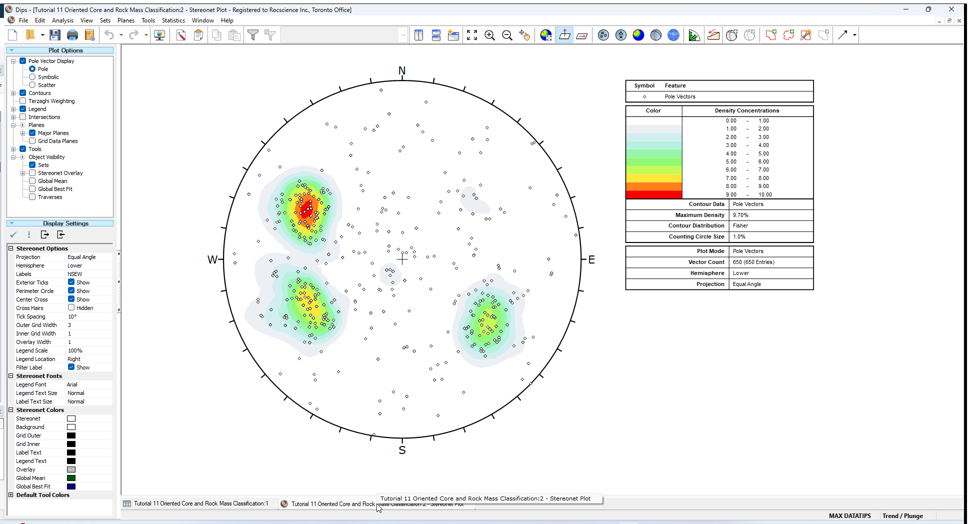
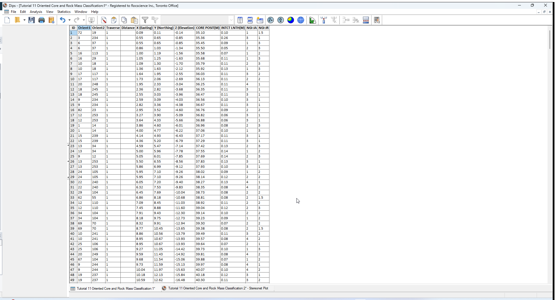
- Switch to the Grid Data view of the file using the view tabs at the lower left.
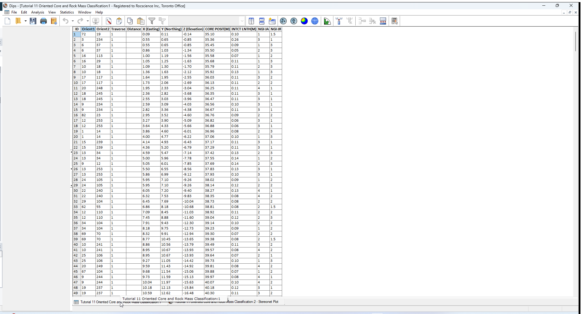
The file contains 650 measurements from 2 oriented borehole cores.
The file uses the following columns:
- The two mandatory Orientation columns
- A Traverse column
- A Distance columns
- Three X (Easting), Y (Northing), Z (Elevation) columns
- 4 Extra Columns
2.1 ORIENTATION COLUMNS
The Orientation Columns for oriented core borehole data record Alpha and Beta core joint angles.
- The Alpha angle, entered in the Orient 1 column, is measured with respect to the core axis.
- The Beta angle, entered in the Orient 2 column, is measured with respect to the core reference line.
2.2 EXTRA COLUMNS
The four Extra Columns record the following information:
- Core position from the borehole collar
- Intact length (calculated in a spreadsheet from position or recorded directly) between adjacent joints
- JA
- JR
The latter measurements are qualitative indices of roughness and alteration taken from the Q Classification by Barton and can be quickly recorded during core logging. Consult any modern rock engineering text for a definition of these terms.
Let’s examine the Project Settings information for this file.
2.3 PROJECT SETTINGS
- Select Project Settings
 from the toolbar or Analysis menu.
 - In the Project Settings dialog:
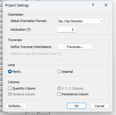
- Note the following:
- The Global Orientation Format = Dip / Dip Direction. However, since we are working with oriented core data, the Global Orientation Format does NOT apply to the data in the Orientation Columns which are Alpha / Beta core angle measurements.
- The Declination = 0 degrees. Declination would, if present, be applied to the borehole trends (azimuths).
- The Quantity Column is not used in this file, so each row of the file represents an individual measurement.
- The Distance Column is selected and disabled. This will be used for the RQD calculation as discussed below.
- The X, Y, Z Columns is selected and disabled.
- Select Cancel to close the dialog.
2.4 TRAVERSES
Let’s inspect the Traverse Information.
- Select the Traverses
 button in the Project Settings dialog (the Traverses option is also available directly in the Analysis menu).
 - In the Traverse Information dialog:
- Select the Linear BH Oriented Core from the Traverse Types list.
- Orient 1 – both traverses have an Orient 1 value of 180. This denotes a reference line (along the length of the core) that is 180 degrees from the top of the core (i.e., at the bottom of the core as it would be in situ).
- Orient 2 – the Orient 2 value indicates the drilling angle from the vertical up direction. Traverse 1 has an Orient 2 value of 135, indicating that the borehole was drilled at 135 degrees from the vertical, or with a plunge of 45 degrees. Traverse 2 was drilled at 160 degrees from the vertical, or a plunge of 70 degrees.
- Orient 3 – the Orient 3 value indicates the azimuth (i.e. clock-wise angle from compass north) of the downhole direction of the borehole. Orient 3 is 40 degrees for Traverse 1 and 135 degrees for Traverse 2.
- Select Cancel in the Traverse Information dialog.
- Select OK in the Project Settings dialog to save the Distance Column checkbox setting.
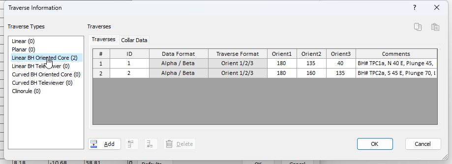
As you can see in the Traverse Information dialog, this file uses two Linear Borehole Traverses. A Linear Borehole Oriented Core Traverse in DIPS requires THREE orientation values in order to fully define the orientation of the borehole and oriented core:
3.0 Distance Column
Notice the Distance column in the spreadsheet (Grid Data view). A Distance column is required if you wish to use any of the following options:
- Joint Spacing
- RQD Analysis
- Joint Frequency
- Curved Boreholes (Oriented Core or Televiewer)
The values in the Distance column should correspond to measurements of joint locations recorded along a Linear or Borehole Traverse.
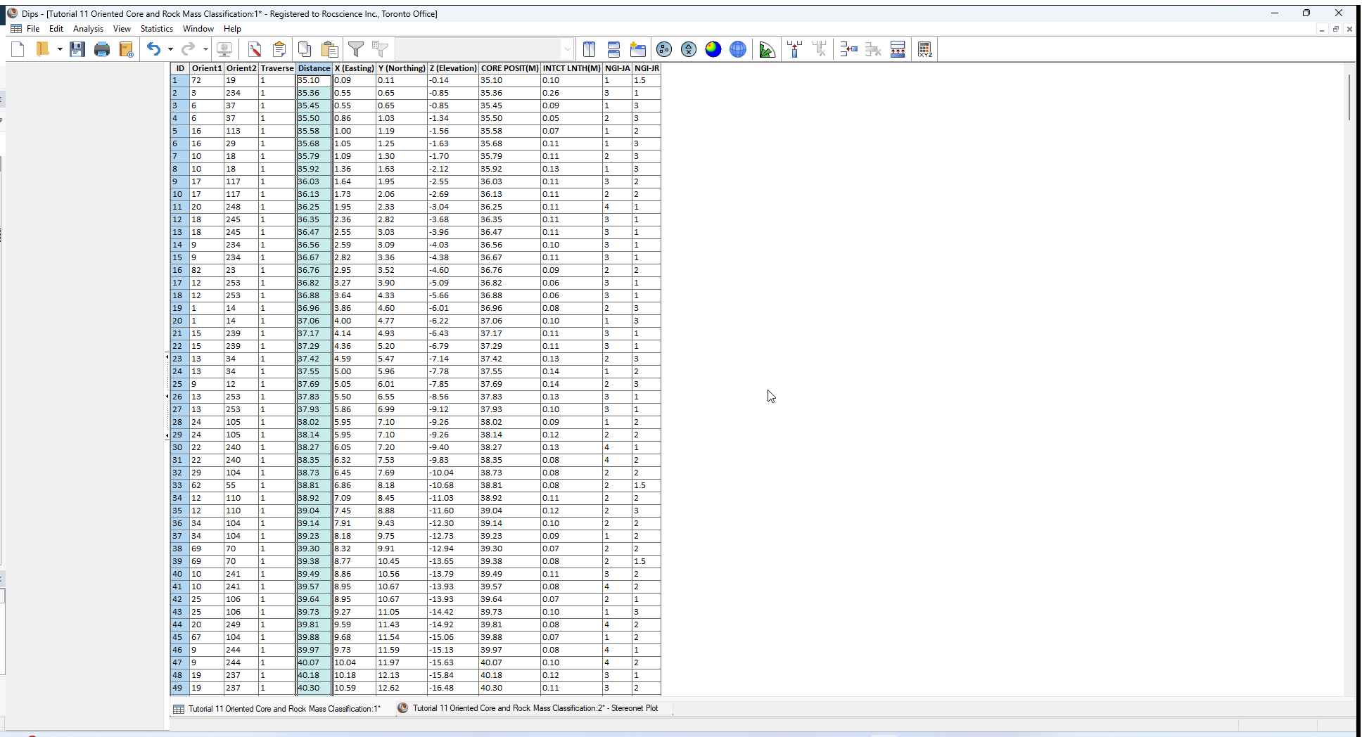
For this example, the Distance values are already recorded in the CORE POSITION column. However, in order for DIPS to recognize the distance data, it must be entered into the Distance column.
So we will simply copy the data in the CORE POSITION column into the Distance column.
- Select the CORE POSITION column by clicking on the column header.
- Select Copy
 from the toolbar, Edit menu, or right-click menu.
 - Select the Distance column by clicking on the column header.
- Select Paste
 from the toolbar, Edit menu, or right-click menu.
 - You should now see the CORE POSITION data duplicated in the Distance column as shown below.
4.0 Rock Tunneling Quality Index – Q
The Rock Tunneling Quality Index, Q, is defined as:
Q = ( RQD / JN ) * ( JR / JA ) * ( JW / SRF )
Consult any modern rock engineering text (see the references at the end of this tutorial) for more information if required.
Set the water parameter JW = 1 (dry) and stress reduction factor SRF = 1 (moderate confinement, no stress problems) for this example.
4.1 DETERMINATION OF Q
The definition of RQD (Rock Quality Designation) is given by:
RDQ = [(Cumulative length of core pieces greater than 10 cm) / (Total length of core)] x 100
We can use the RQD Analysis option to automatically calculate RQD along the lengths of the Traverses, from the values in the Distance column.
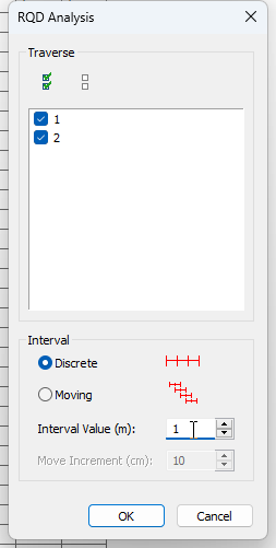
- Select RQD Analysis from the Analysis menu.
- In the RQD Analysis dialog:
- Select the checkboxes for Traverse 1 and 2.
- Set Interal = Discrete.
- Enter Interval Value = 1 m.
- Select OK.
You should see the graph below. 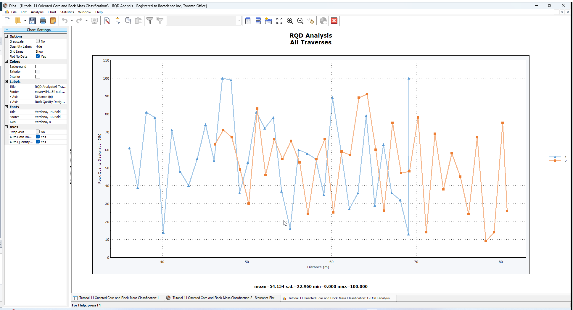
Using the values in the Distance column, RQD is automatically calculated along the length of the selected Traverses.
NOTE:
- The data for the two Traverses are plotted separately on the graph.
- At the bottom of the graph, statistics are displayed. This shows the mean, standard deviation, min and max values, based on ALL RQD values calculated for all selected traverses.
In this case, the mean RQD value = 54% which we will use in the calculation of the Q index.
4.2 DETERMINATION OF JN
JN is the joint number. To obtain a value for this parameter, let’s view a Contour Plot, to determine the number of (well) defined joint sets.
- Select the Contour Preset
 toolbar button.
 - Select the Terzaghi Weighting checkbox in the Sidebar Plot Options.
Applying Terzaghi Weighting will allows us to view the weighted contours.
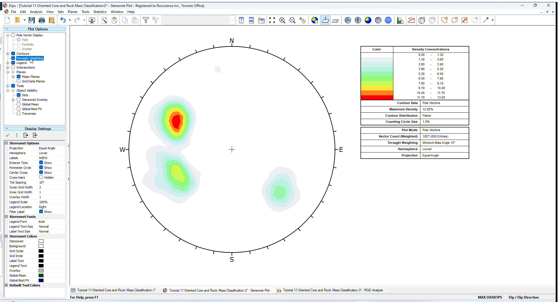
The three well defined joints sets result in Barton’s JN = 9.
Now use Add Set Window ![]() option to determine the mean orientations of the three joint sets. (See Tutorial 03 - Sets (Set Window)) for details about creating Sets with the Add Set Window
option to determine the mean orientations of the three joint sets. (See Tutorial 03 - Sets (Set Window)) for details about creating Sets with the Add Set Window ![]() option.)
option.)
- Select Add Set Window
 option from the toolbar to create Set 1.
 - Click, drag, and click the mouse to encompass the poles at the upper left of the stereonet.
- In the Add Set Window dialog:
- Enter First Corner Dip / Dip Direction = 46 / 93.
- Enter Second Corner Dip / Dip Direction = 84 / 139.
- Select OK.
- Select Add Set Window option from the toolbar to create Set 2.
- Click, drag, and click the mouse to encompass the poles at the lower left of the stereonet.
- In the Add Set Window dialog:
- Enter First Corner Dip / Dip Direction = 46 / 41.
- Enter Second Corner Dip / Dip Direction = 81 / 91.
- Select OK.
- Select Add Set Window option from the toolbar to create Set 3.
- Click, drag, and click the mouse to encompass the poles at the lower right of the stereonet.
- In the Add Set Window dialog:
- Enter First Corner Dip / Dip Direction = 50 / 287.
- Enter Second Corner Dip / Dip Direction = 78 / 328.
- Select OK.
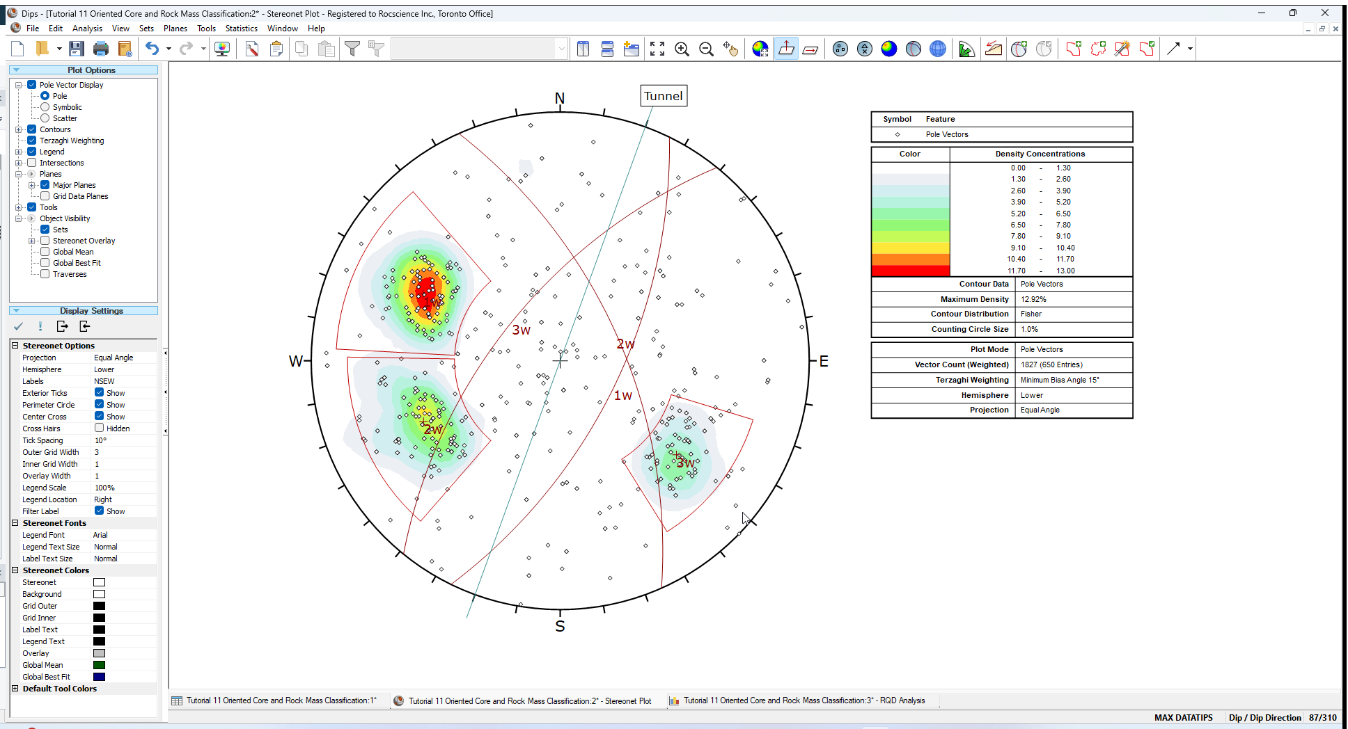
Finally, let’s add a LINE through the center of the stereonet, to represent a proposed tunnel axis. Assume a tunnel trend of 20 degrees.
- Select Trend Line
 option from the Tools menu.
 - Place the cursor at APPROXIMATELY Trend = 20 degrees, and click the left mouse button (remember that the cursor coordinates are visible in the Status Bar).
- In the Add Trend Line dialog:
- If your graphically entered orientation is not exactly 20 degrees, then enter Trend = 20 degrees.
- Select OK.
- Select Pole Vector Display > Poles checkbox in the Sidebar Plot Options.
- Use the Add Text
 tool to add the label Tunnel to the trend line.
 - Superimpose the tunnel axis on the Mean Set Planes to judge the critical joint set for Q classification.
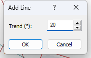
It is not immediately obvious which is the critical joint in this case. However, it can be shown that joint Set 1 is most likely to prevent any development of tension in the roof and therefore will reduce the self-supporting nature of the tunnel roof. Let us then use this as the critical joint set for Q classification. Note the sliding wedge (closed triangle in the above plot formed by the three joint sets) which appears in the roof of the tunnel.
4.3 ESTIMATION OF JR AND JA
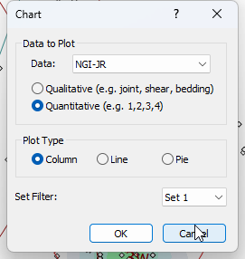
The next step is to use the Chart option to look at JR and JA. These indices can be viewed as either Qualitative or Quantitative. Quantitative Analysis allows a mean calculation and so is preferred.
- Select Analysis > Chart
 from the menu.
 - In the Chart dialog:
- Select Data = NGI-JR.
- Select Data to Plot = Quantitative radio button.
- Set Set Filter = Set 1 in the dropdown.
- Select OK.
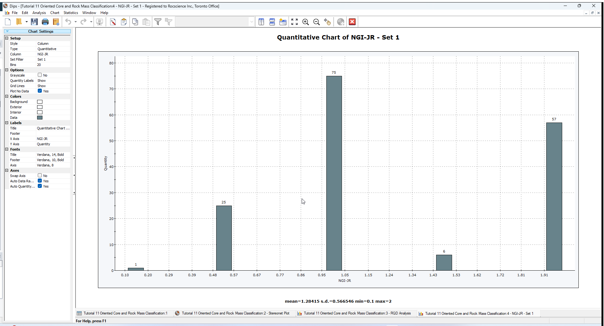
Notice the mean and standard deviation at the bottom of the Chart. The mean value of JR is approximately 1.3.
Now change the data type to NGI-JA.
- In the Sidebar Chart Settings > Setup select Column = NGI-JA
- Make sure the Type = Quantitative.
The mean value of JA is approximately 3.2.
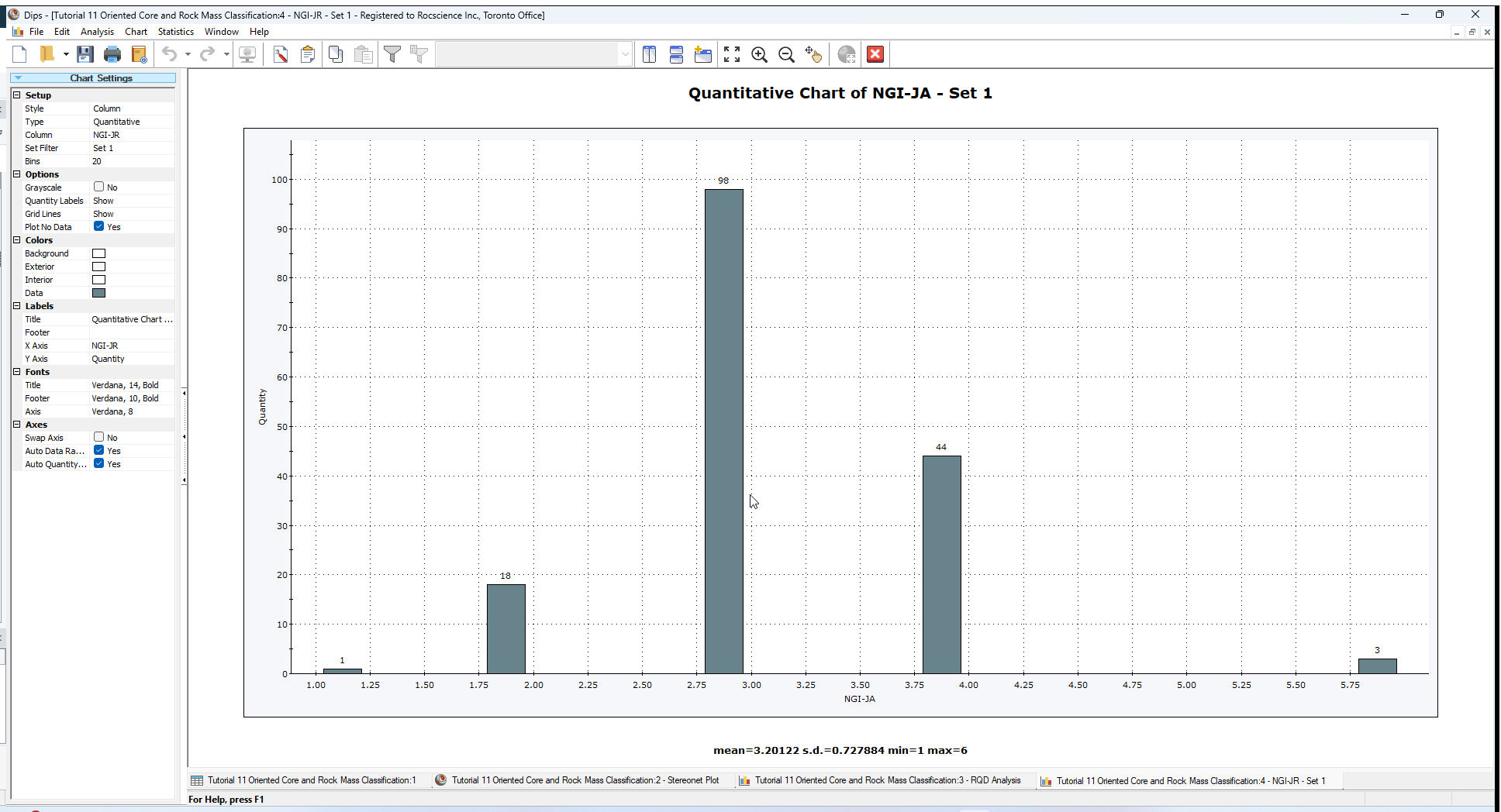
For the purposes of classification, a JR of 1 to 1.5 and a JA of 3 to 4 would be adequate in this example.
4.4 CALCULATION OF Q VALUES
RQD, as calculated above was 54%. Using the JN value of 9, and the upper and lower limits for JR and JA (see above), gives:
- A lower Q of ( 54 / 9 ) * ( 1 / 4 ) * ( 1 / 1 ) = 1.5
- An upper Q of ( 54 / 9 ) * ( 1.5 / 3 ) * ( 1 / 1 ) = 3
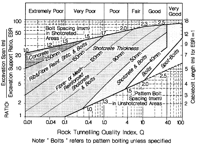
This range of values can now be used for further empirical support design according to Barton’s design charts; see the figure below. Real values for JW may be evaluated qualitatively from borehole inflow notes. SRF can be determined from the depth of the proposed excavation according to Barton.
Tunneling support guidelines, based on the tunneling quality index Q (bolt lengths modified for cablebolting). Ref. [1], after original Ref. [3].
5.0 Display of Traverses
Finally, we will point out a useful display option to show Traverses on the stereonet.
- Go back to the Stereonet Plot view.
- Select the Traverses checkbox in the Sidebar Plot Options.
The Traverse orientations will be displayed on the stereonet.
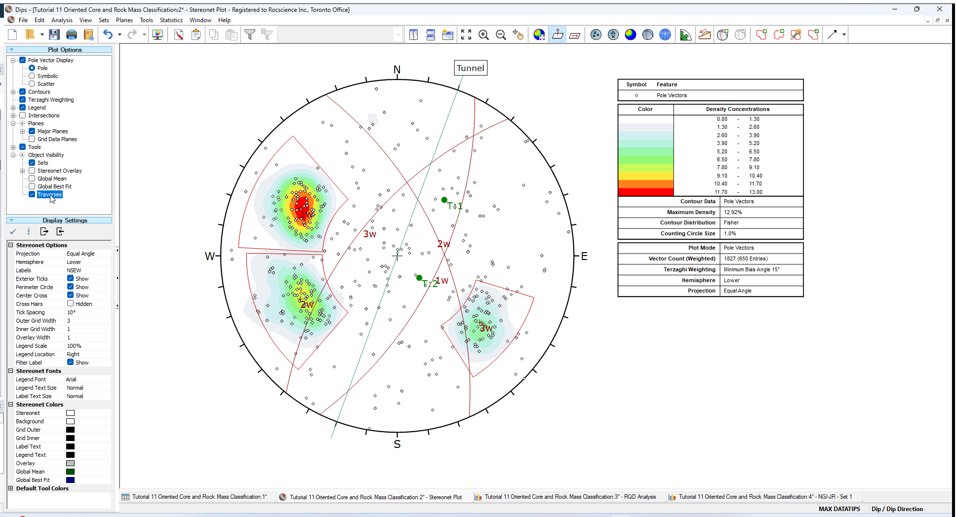
You can now see the two borehole orientations plotted on the stereonet (green circles with Traverse ID). The symbols used to display the Traverses can be customized in the Symbol Editor dialog (Edit > Edit Symbols).
6.0 Frequently Asked Borehole Traverse Questions
To conclude this tutorial we will answer 3 frequently asked questions regarding borehole Traverse and oriented core data processing with DIPS.
- How do I obtain a listing of true Dip / Dip direction values from oriented core data?
- Can I define a curved borehole in DIPS?
- I already have processed borehole data from televiewer measurements (e.g., direct measurement of fracture orientations by optical or acoustic televiewer). What type of Traverse do I use in DIPS?
ANSWER: If the borehole is linear you can use either the Linear or Linear BH Televiewer Traverse options (these are equivalent, you may use either option). If the borehole is non-linear then use the Curved BH Televiewer Traverse option.
ANSWER: Use the Process Data option in the Analysis menu and save a new DIPS file in the processed format of your choice.
ANSWER: Yes; there are two new Traverse options – Curved BH Oriented Core and Curved BH Televiewer. These options allow you to enter Survey File data for non-linear boreholes.
See the Traverse Types topic for further information.
7.0 References
- Hutchinson, D.J. and Diederichs, M. 1996. Cablebolting in Underground Mines, Vancouver: Bitech. 400 pp.
- Hoek, E., Kaiser, P.K. and Bawden, W.F. 1995. Support of Underground Excavations in Hard Rock. Rotterdam: Balkema.
- Grimstad, E. and Barton, N. 1993. Updating the Q-System for NMT. Proc. int. symp. on sprayed concrete - modern use of wet mix sprayed concrete for underground support, Fagernes, (eds Kompen, Opsahl and Berg). Oslo: Norwegian Concrete Assn.
This concludes the tutorial. You are now ready for the next tutorial, Tutorial 12 - Joint Spacing, RQD, and Joint Frequency in DIPS.