12 - Joint Spacing, RQD, Frequency
1.0 Introduction
This tutorial will demonstrate how to use the Joint Spacing, RQD and Joint Frequency analysis options in DIPS. The tutorial uses the example file Joint Spacing.dips8 which is set up for such analyses.
Topics Covered in this Tutorial:
- True Joint Spacing
- RQD Analysis
- Joint Frequency
- Core Loss
Finished Product:
The finished product of this tutorial can be found in the Tutorial 12 Joint Spacing RQD Frequency.dips8 file, located in the Examples > Tutorials folder in your DIPS installation folder.
2.0 Model
If you have not already done so, run DIPS by double-clicking on the DIPS icon in your installation folder. Or from the Start menu, select Programs > Rocscience > DIPS > DIPS.
If the DIPS application window is not already maximized, maximize it now, so that the full screen is available for viewing the model.
DIPS comes with several example files installed with the program. These example files can be accessed by selecting File > Recent Folders > Examples Folder from the DIPS main menu. This tutorial will use the Joint Spacing.dips8 file to demonstrate the basic plotting features of DIPS.
- Select File > Recent Folders > Example Folder
 from the menu.
 - Open the Joint Spacing.dips8 file. Since we will be using the Joint Spacing.dips8 file in other tutorials, save this example file with a new file name without overwriting the original file.
- Select File > Save As
 from the menu.
 - Enter the file name Tutorial 12 Joint Spacing RQD Frequency and Save the file.
You should see the stereonet plot view shown in the following figure.
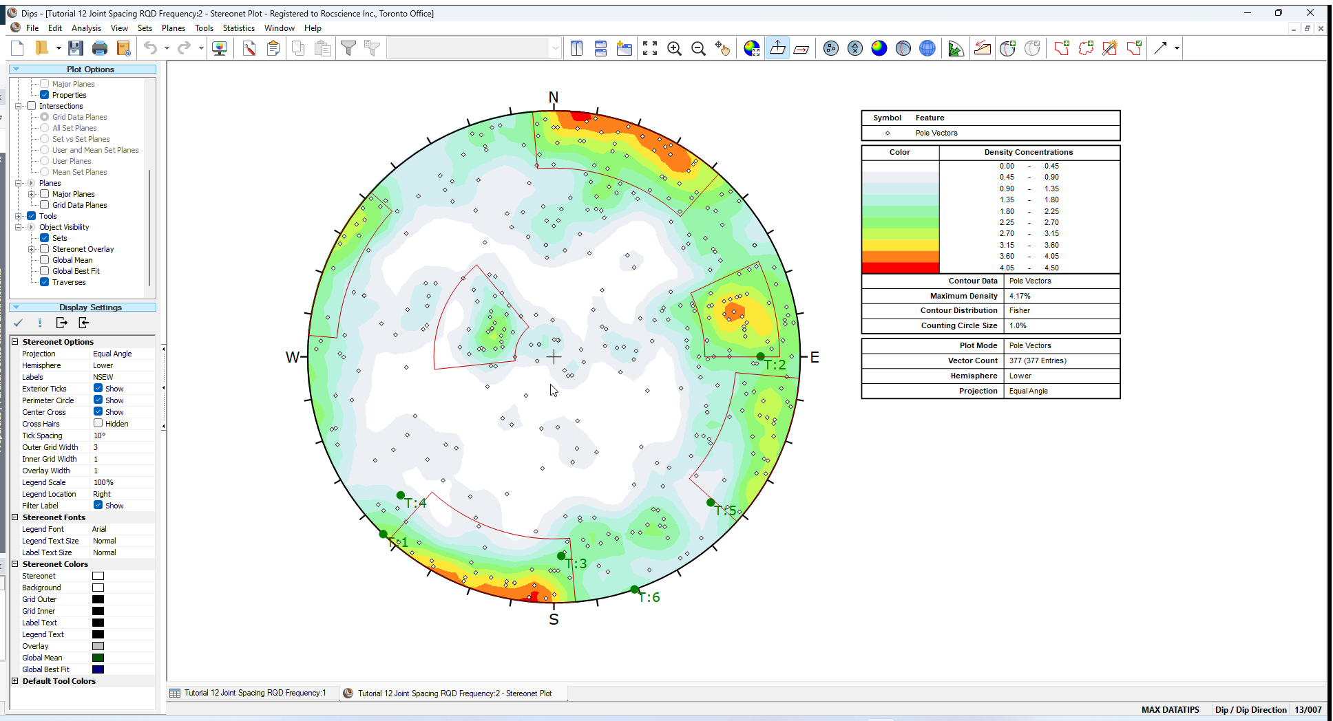
The main features of this file are:
- Six Linear traverses are defined (Analysis > Traverses).
- The Distance Column is enabled and Distance measurements along each Linear Traverse have been entered.
In addition, for convenience, four Set Windows defining four joint sets, have already been added over the main pole concentrations on the stereonet.
2.1 PROJECT SETTINGS
- Select Project Settings
 from the toolbar or the Analysis menu.
 - In the Project Settings dialog:
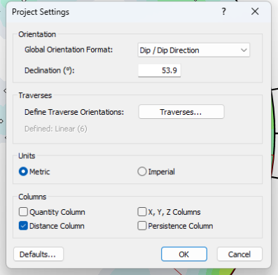
Note the following:- The Global Orientation Format = Dip/Dip Direction
- The Declination = 53.9 degrees, indicating that 53.9 degrees will be added to the dip direction of the data, to correct for magnetic declination
- The Distance Column is used in this file.
- The Units = Metric.
- Select Cancel to close the dialog.
3.0 Distance Units
The Units for the Distance Column are selected in Project Settings, either Metric (meters) or Imperial (feet). In this case, the Units = Metric (meters).
The Units apply to the Distance column and all related analyses (e.g., Joint Spacing, RQD, Joint Frequency).
4.0 Joint Spacing
The Joint Spacing option will convert distance measurements along a linear or borehole Traverse, into true (perpendicular) spacings between adjacent joints belonging to the same joint set.
The figure below illustrates the geometry in 2D; the actual calculation accounts for the 3-dimensional orientations of the planes with respect to the Traverse line.
The Joint Spacing option is only enabled if THREE criteria are met:
- You must have at least one (or more) joint sets defined, using the options available for creating sets (e.g. Add Set Window, Add Set Freehand).
- You must have at least one (or more) linear or borehole traverses defined (e.g. Linear, Linear BH Oriented Core, Linear BH Televiewer, Curved BH Oriented Core, Curved BH Televiewer).
- The Distance Column must be enabled (checkbox in Project Settings) and Distance values entered.
The Joint Spacing.dips8 file that you have just opened, satisfies the above criteria, so we will proceed to the Joint Spacing option.
- Select Analysis > Joint Spacing from the menu.
- In the Joint Spacing dialog:
- Set Spacing = True Spacing.
- Select Set = 1.
- Select All Traverses (select the Select All
 button).
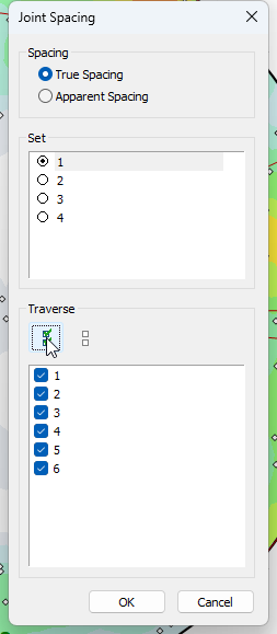
- Select OK.
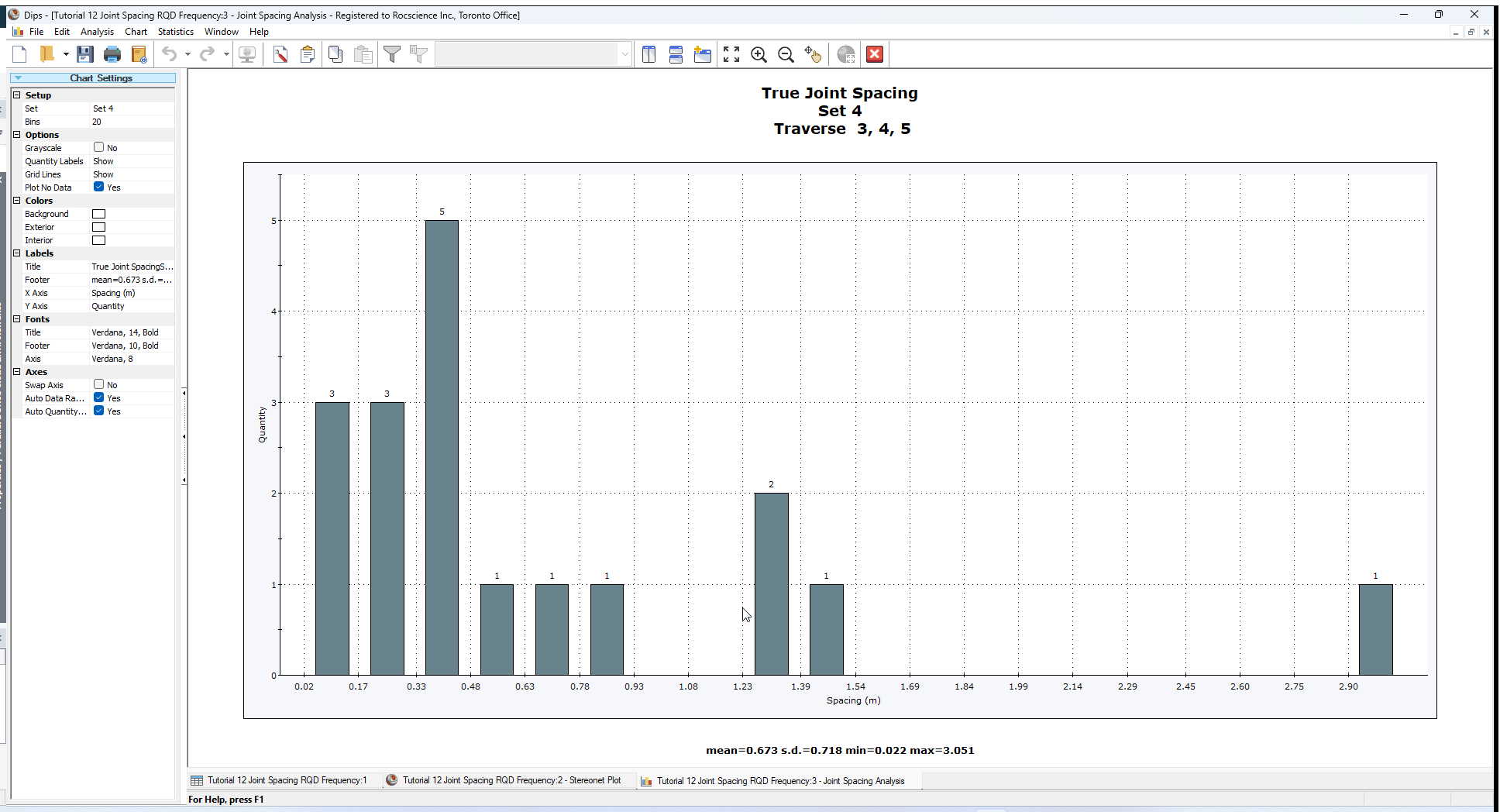
You should see the following graph.
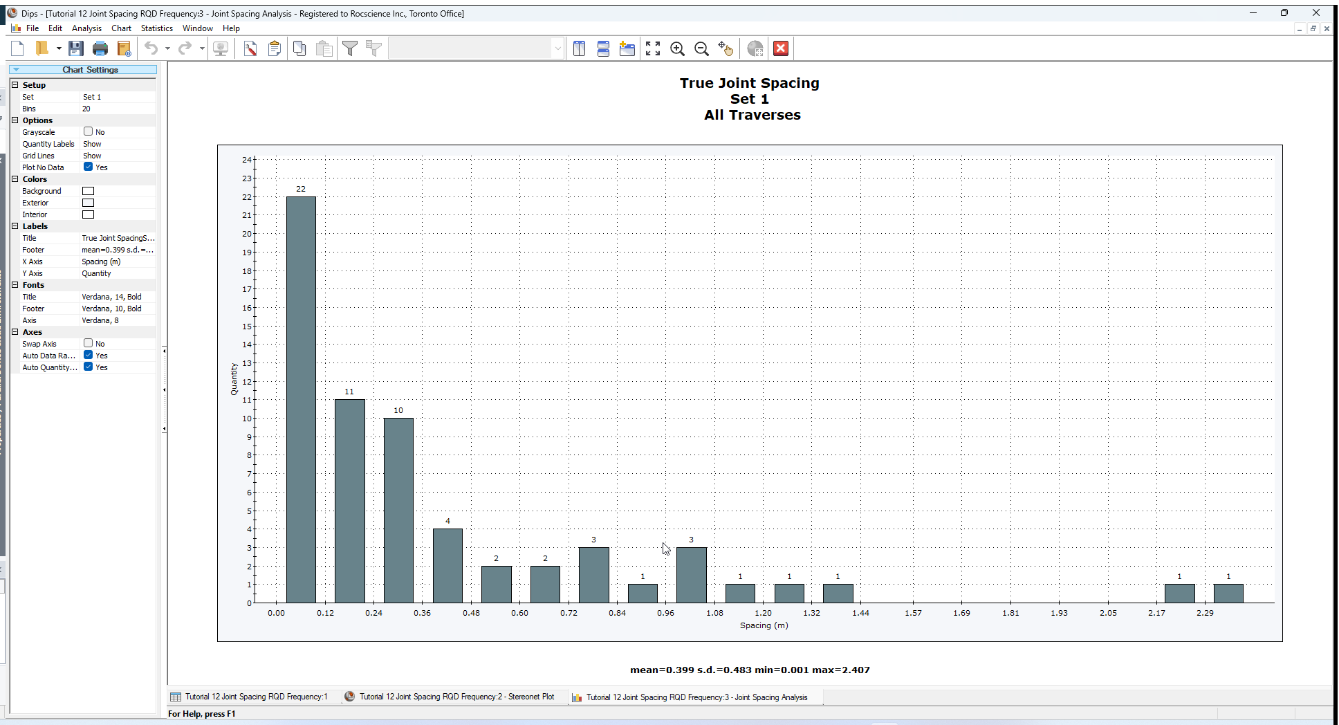
This plots the distribution of true joint spacing for Set 1, using data from All Traverses. The mean, standard deviation, min. and max. values are listed at the bottom of the plot.
4.1 SETS
Once a Joint Spacing graph has been generated, for convenience, you can choose which Set to plot from the Sidebar Chart Settings. This will update the graph within the active chart view.
Choose different Sets and view the resulting graphs.
4.2 TRAVERSES
If you wish to plot data using Select Traverses, then you will have to return to the Joint Spacing option in the Analysis menu.
- Select Analysis > Joint Spacing from the menu.
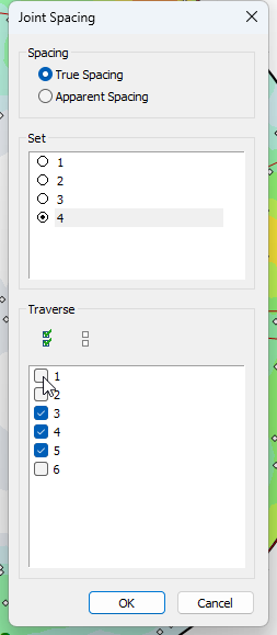
- In the Joint Spacing dialog:
- Select Set = 4.
- Select Traverses 3, 4, and 5.
- Select OK to generate a new plot.
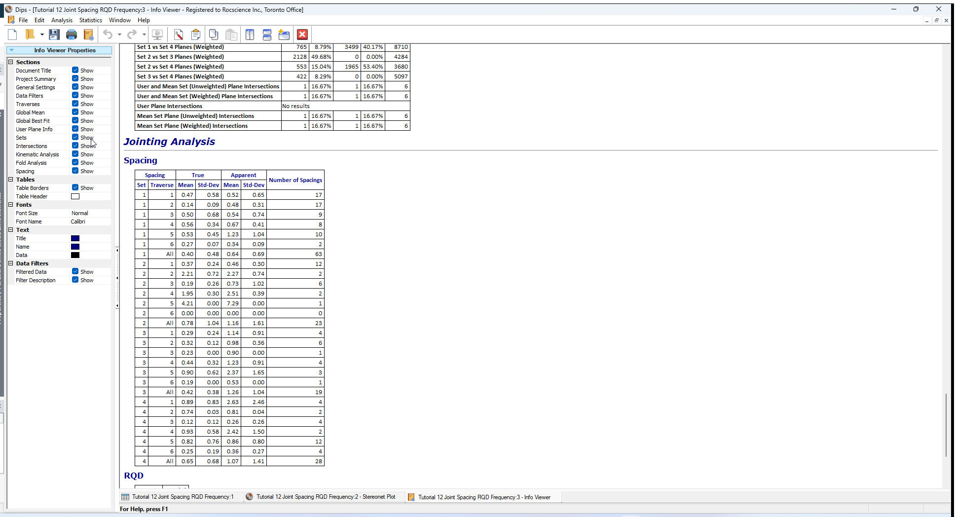
4.3 INFO VIEWER
The Info Viewer presents a summary of joint spacing statistics for each Traverse and Set combination, and for each set using all Traverses.
- Select Info Viewer
 from the toolbar or Analysis menu.
 - Scroll down to the Jointing Analysis section of the Info Viewer.
5.0 RQD Analysis
Now let’s demonstrate the RQD Analysis option.
The RQD Analysis option allows you to calculate the Rock Quality Designation (%) calculated from distance measurements recorded along a linear or borehole Traverse. When adjacent distance measurements between joints are less than or equal to 10 centimeters (metric) or 4 inches (imperial), that length is flagged as "poor quality". RQD is a measure of the percentage of core length pieces which are greater than this cutoff value, relative to the total measured interval.
In order to use the RQD Analysis option:
- You must have at least one (or more) Linear or Borehole Traverses defined (e.g. Linear, Linear BH Oriented Core, Linear BH Televiewer, Curved BH Oriented Core, Curved BH Televiewer).
- The Distance Column must be enabled (checkbox in Project Settings) and distance values entered.
The Joint Spacing.dips8 file that you have just opened, satisfies the above criteria, so we will proceed to the RQD Analysis option.
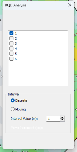
- Select RQD Analysis from the Analysis menu.
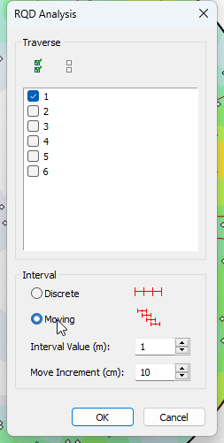
- In the RQD Analysis dialog:
- Select Traverse = 1.
- Select Interval = Discrete.
- Enter Interval Value = 1 m.
- Select OK.
You should see the following graph for Traverse 1.
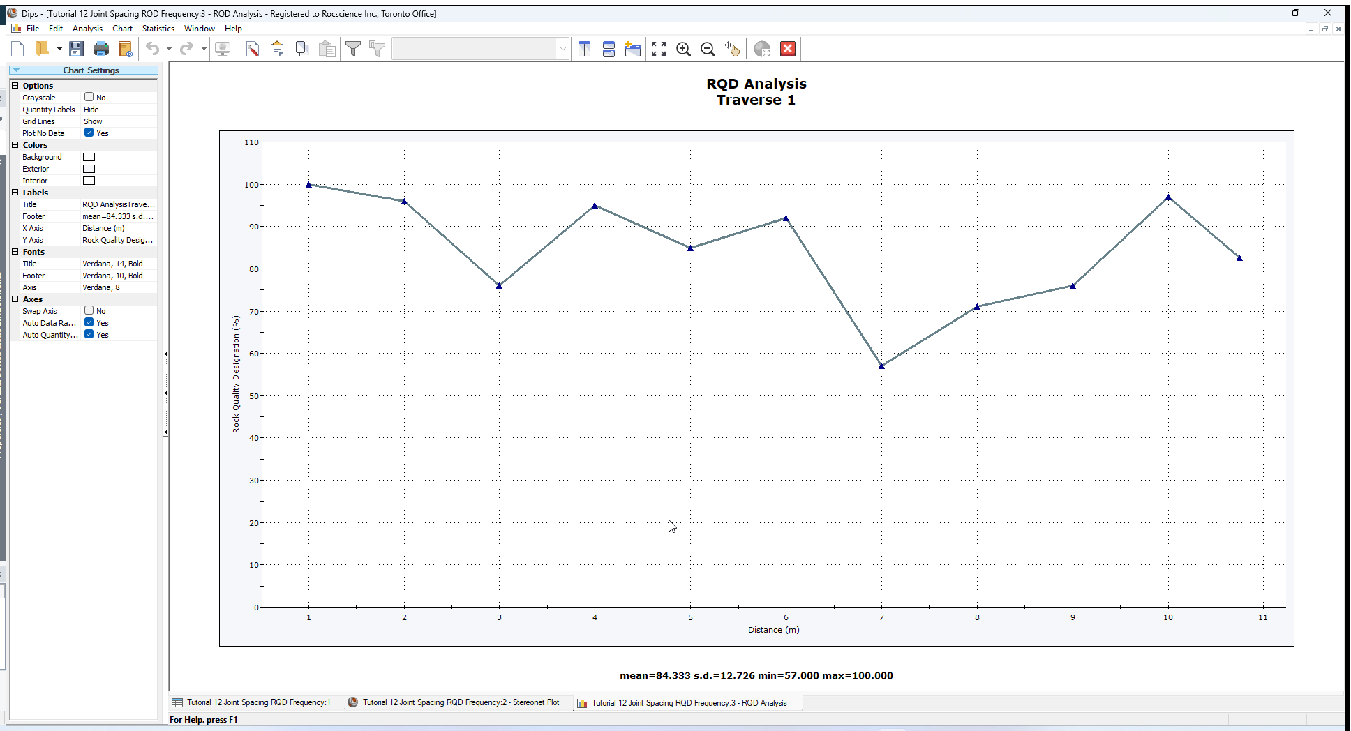
With the Discrete interval option, each interval begins at the end of the previous interval.
Let’s try the Moving Interval option, which moves the interval in overlapping increments. This may help to better identify narrow transitions in RQD value.
- Select Analysis > RQD Analysis from the menu.
- In the RQD Analysis dialog:
- Select the Interval = Moving
- Use the default interval (Interval Value = 1 m) and increment (Move Increment = 10 cm) values.
- Select OK.
You should see the following graph for Traverse 1.
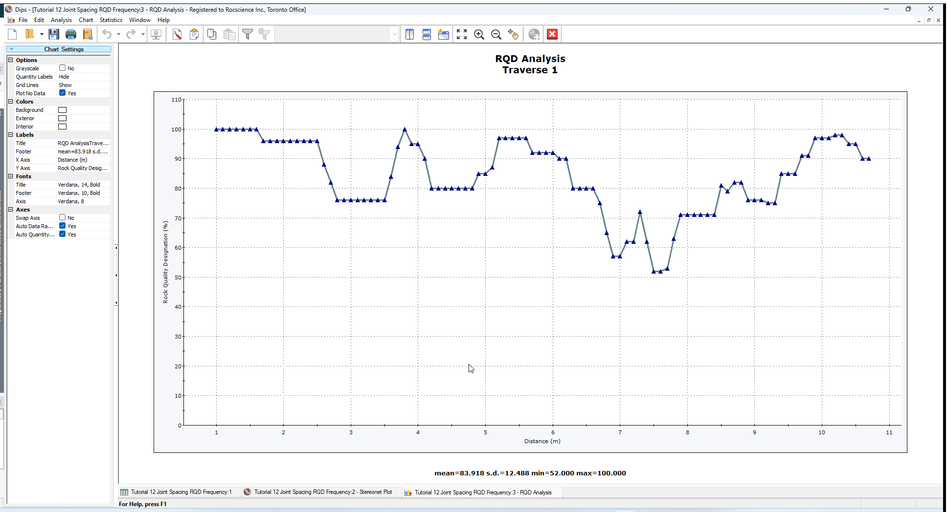
You can also plot multiple Traverses on the same RQD plot, this is left as an optional exercise.
6.0 Joint Frequency
The Joint Frequency option is very similar to the RQD Analysis option, and allows you to plot the linear 1D frequency of joints along the length of each Traverse.
In order to use the Joint Frequency option:
- You must have at least one (or more) linear or borehole traverses defined.
- The Distance Column must be enabled (checkbox in Project Settings) and distance values entered.
The Joint Spacing.dips8 file that you have just opened, satisfies the above criteria, so we will proceed to the Joint Frequency option.
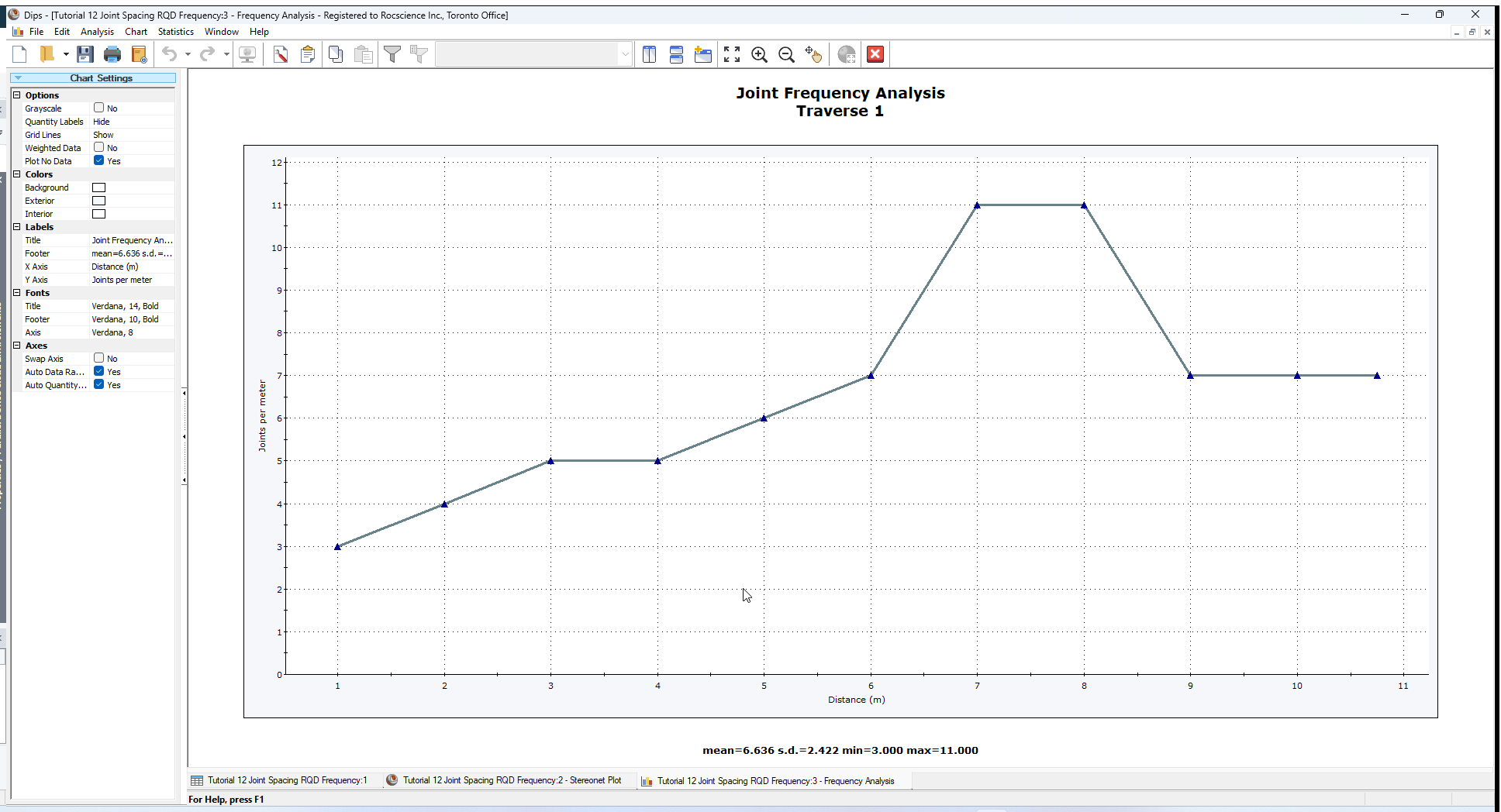
- Select Joint Frequency from the Analysis menu.
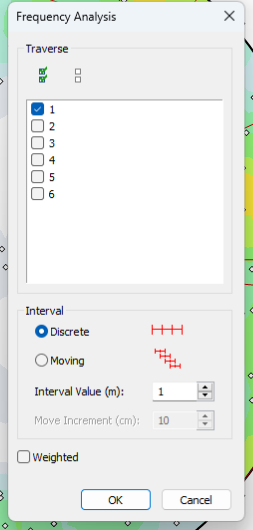
- In the Frequency Analysis dialog:
- Select Traverse = 1.
- Select Interval = Discrete.
- Enter Interval Value = 1 m.
- Select OK.
You should see the following graph for Traverse 1.
You can also apply the Terzaghi Weighting to the Joint Frequency.
- Select Analysis > Joint Frequency from the menu.
- In the Frequency Analysis dialog:
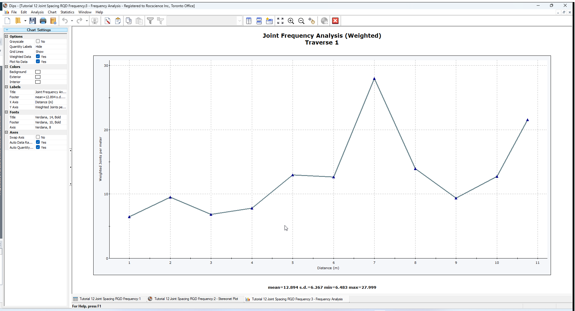
- Select the Weighting checkbox. This will apply the Terzaghi Weighting to the joint count, and plot the weighted number of joints per meter.
- Select OK.
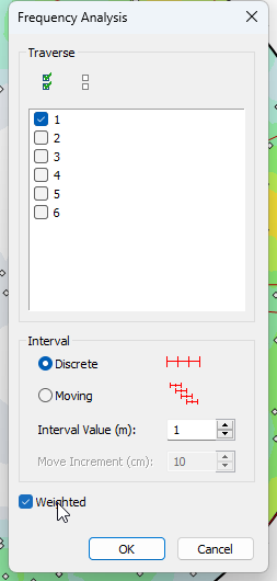
You should see the following graph for Traverse 1.
7.0 Core Loss
It should be noted that the Jointing Analysis options do not account for intervals of lost or damaged core or unlogged core. It is assumed that distance readings are from continuous measurement of intact core.
This has the following implications:
- Joint Spacing – for the Joint Spacing option, if there is a gap in the Distance measurements, it is possible that an artificially large joint spacing value may be recorded, if joints from a given set occur on either side of a gap.
- RQD – for the RQD option, a gap in distance measurements would be recorded as RQD = 100, since no joints would be recorded, which would register as “intact” core.
- Joint Frequency – for the Joint Frequency option, frequency would be recorded as zero over a gap in the distance record.
In conclusion, there is currently no method of specifying lost/damaged/unlogged core lengths for the Jointing Analysis options, so this should be kept in mind when interpreting results.
This concludes the tutorial. You are now ready for the next tutorial, Tutorial 13 - Curved Boreholes.