Density Calculation
In the Contour Options dialog, the following options are available which control the way that Dips computes the pole density concentration values for the data:
- Fisher Distribution
- Schmidt Distribution
- Count Circle Size
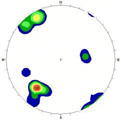
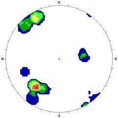
The Schmidt distribution method provides very quick computation time and, for large amounts of data, produces concentration values which are very similar to those obtained with the Fisher method. When the quantity of data is limited, however, the Schmidt distribution produces very crude contour diagrams and often misleading results, since each measurement is assumed to be 100 percent accurate and any existing errors are exaggerated due to lack of data. Therefore in this case, it is advisable to use the Fisher distribution, since it tends to suppress any undue influence that a single measurement might have on the data contained in a limited data set. When you have lots of data, there is little difference between the plots generated by the two methods, and the Schmidt distribution is faster.
Contour plot using Fisher distribution, 40 points in data set |
Contour plot using Schmidt distribution, 40 points in data set |
Fisher Distribution
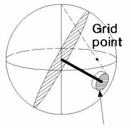
In the Fisher method each pole is assigned a normal influence or Fisher distribution over the surface of the sphere, rather than a point value, as in the Schmidt method. The integrated zone of influence is a bell shaped distribution with a maximum height of 1, and a basal radius twice that of the counting circle radius. The influence contribution to a grid point is represented by the height of the influence zone immediately above the grid point. In this method, the total influence of an individual pole is the same as in the Schmidt method but its distribution of influence reflects an assumed probability of measurement error. For large quantities of data, this option will produce similar results to the familiar Schmidt option. The real strength of the Fisher option is in "smoothing" density plots for sparse data sets.

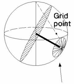
Bell dome of influence: maximum height = 1 coincident with pole vector. Base radius = 2 x Schmidt cylinder radius. Total volume of influence function is equal to Schmidt cylinder.
Schmidt Distribution
The Schmidt distribution is the classical method, in which each pole is assigned a constant influence value of 1. The integrated zone of influence is a cylinder of constant height with a radius equal to the radius of the counting circle. A counting grid is superimposed on the stereonet plane, or in the case of Dips, on the surface of the reference sphere. Convention dictates the use of a counting circle with an area equivalent to 1% of the lower hemisphere surface. For each pole plotted, any grid point falling within a circle of arbitrary constant radius centered on this pole is incremented by the value of the pole. After the influence of all plotted poles is thus distributed, the density plotted at each grid point is calculated by dividing the pole count at that grid point by the total pole influence.

Cylinder of influence: Height = 1
Count Circle
In the Contour Options dialog, you can customize the Count Circle Size used in the contour calculations.
The generally accepted Count Circle Size used in contour calculations is one percent of the surface area of the lower reference hemisphere. This is, however, merely convention and if desired, you may use a different Count Circle Size. The allowed range of count circle area as a percentage of hemisphere area is 0.5 % to 5.0 %. For meaningful results, a range limit of 1.0 % to 2.5 % is recommended.

