Comparison of load-settlement curves from an O-Cell test with pile analysis using T-z curves
By Ahmed Mufty, Ph.D., P.Eng.
Introduction
The bi-directional axial compressive load test BDSLT which is traditionally known as O-Cell test is conducted on bored piles by embedding a hydraulic jack (O-Cell) within a pile body. The test is usually fully instrumented with telltales and strain gauges to measure displacements and strains along the pile length. With the recorded strains and displacements at different loading levels, the pile capacity and response to loading may be estimated conveniently.
This article is devoted to showing how T-z curves obtained from the test may be used to determine the expected settlement for working piles. A comparison is made between the results obtained from the traditional construction of the top load test, TLT, using O-Cell test data with the settlement response estimated using software like RSPile applying the T-z curves deduced from the interpretation of the test results.
From an actual BDSLT that was conducted on a pile embedded in sandstone, the test results are interpreted and used for this study. The end bearing resistance was eliminated and the O-Cell was installed at the middle of the pile length. A T-z curve for the sandstone will be chosen from the obtained records and applied in RSPile axial pile analysis. If needed, suitable multipliers may be applied to adjust the applied curve to make the results ready for analysis of working piles.
Ground Layers
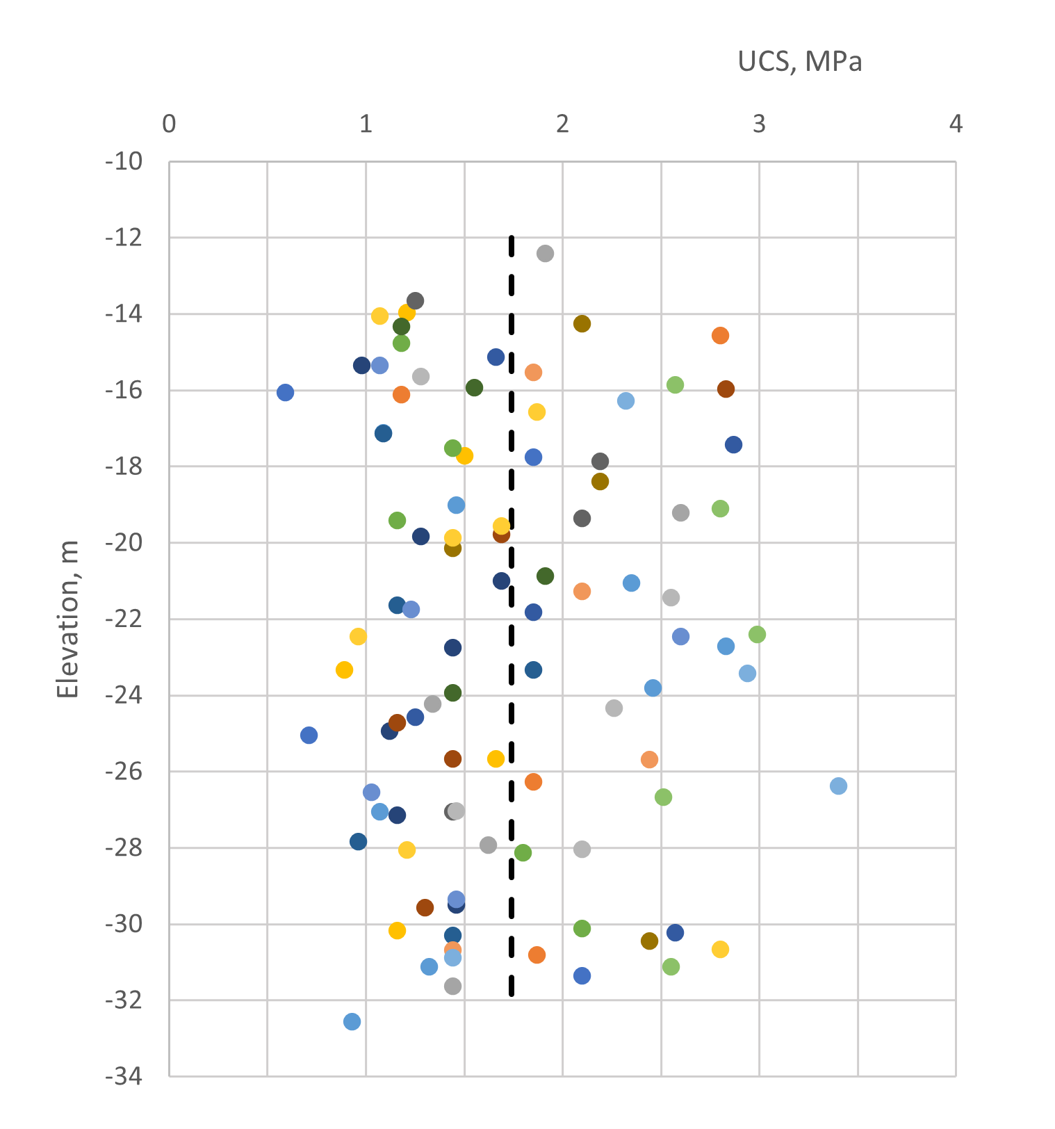
The ground layers are composed of medium dense sand overlaying a deep and very weak sandstone layer. Based on the reference levels of the local area the ground surface was at +3m. The SPT blow count obtained from 19 boreholes showed that the deepest elevation possible for the sand layer was at -12m. in the project area. The average rock quality designation, RQD, for the rock was found to be 65%. The unconfined compressive strength of the rock layer is plotted against depth in Fig.1, with an average of 1.74 MPa. With these figures, the ultimate pile skin friction may be calculated using RSPile “Bored” mode. The applied methods showed the following results:
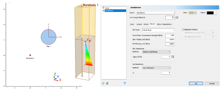
Williams and Pells method gave 504 kPa while Kulhawy and Phoon Method resulted in a unit ultimate skin resistance of 295 kPa, 589 kPa and 885 kPa for c values of 1, 2, and 3 respectively. Refer to RSPile theory manual. The modeled pile was of 1m diameter and 12m length embedded in sandstone having the properties given above. The concrete cylinder strength was 40MPa. The reader can easily model the soils and the pile to get these results, see Fig.2.
Details of the Test Pile
The 12m pile is divided in the middle by the O-Cell as shown in Fig.3. The top and the bottom parts are of 6m length each. The top part is supposed to have no resistance to the load at the top as the hole is kept empty of any fill and the bottom base of the pile is cast on a Styrofoam which will ensure no end bearing resistance. The top pile and the bottom pile are instrumented with strain gauges at the levels shown, while the pile head, cell top, and bottom plates are connected to telltales to measure the movement at these points. When the test starts the jack load will be equally applied to both parts pushing the top pile upward and the bottom pile downward.
The original pile length is 12m and supposed to hold a load of 6000 kN. Hence, the jack load representing the design load will be 3000 kN in each direction. The test will continue till failure to reach the ultimate skin resistance as the first part fails or both parts if they fail simultaneously. Because of the over concreting at the top, it may be expected that the bottom part will fail first and that is what happened in the test. The level of the concrete at the top head might not be controlled accurately. Anyhow, the pile segments closer to the O-Cell will be almost having the same skin resistance.
The pile is 1m in diameter and the section is reinforced with 16-25mm steel bars having a modulus of elasticity of 200 GPa while the concrete modulus is estimated from cylinder strength to be around 31 GPa leading to a modular ratio n of 6.45. With this modular ratio, the equivalent modulus of the composite section of the pile may be calculated as 𝐸𝑝=𝐸𝑐 (1−𝜌+𝑛𝜌) where 𝜌 is the reinforcement steel ratio As/Ag and hence equals to 32690 MPa.
The maximum average stress allowed during the test should keep the pile within elastic ranges. The maximum load applied during the test was around 13000 kN which is equivalent to an average stress of 16.56 MPa (around 40% of the concrete strength during the test). This figure is still high and some nonlinearity may be expected in the concrete behavior at the maximum test load.
Test results and traditional TLT load settlement curve.
The test was conducted following the ICE SPERW testing schedule for static load tests of trial piles. The O-Cell test procedure is now standardized in ASTM D8169-2018. Table 1 lists the microstrain (strain x 1E6) values recorded from the strain gauges corresponding to the jack loading stages and elevations. The strains at Cell top and bottom are calculated based on the load applied and the equivalent modulus for the composite section given above.
In table 2, the recorded displacements at the head of the top pile and at the cell level are listed against the loading stages.
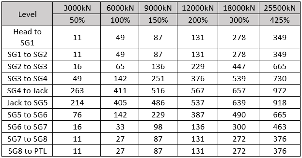
With the strains available from Table 1, it is easy to calculate the mobilized skin friction for each segment of the pile in every load step. The skin friction values are listed in Table 3. The values are plotted in Fig.4 against the absolute displacement which in turn are computed from the displacements given in Table 2 and the strain differences.
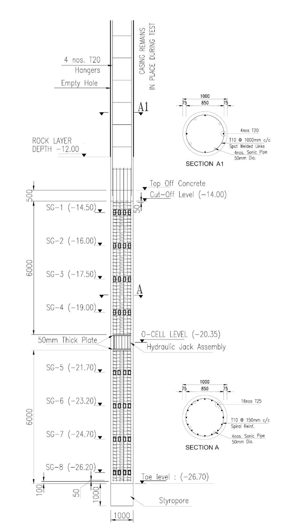
Table 1: Strain measurements during the test
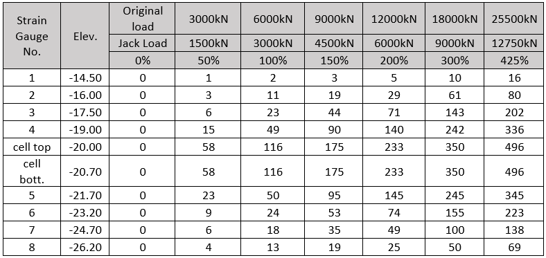
Table 2: Displacements during the test at end of each load stage (unloading is not listed)
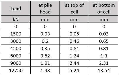
Table 3: Unit skin resistance mobilized at each load step
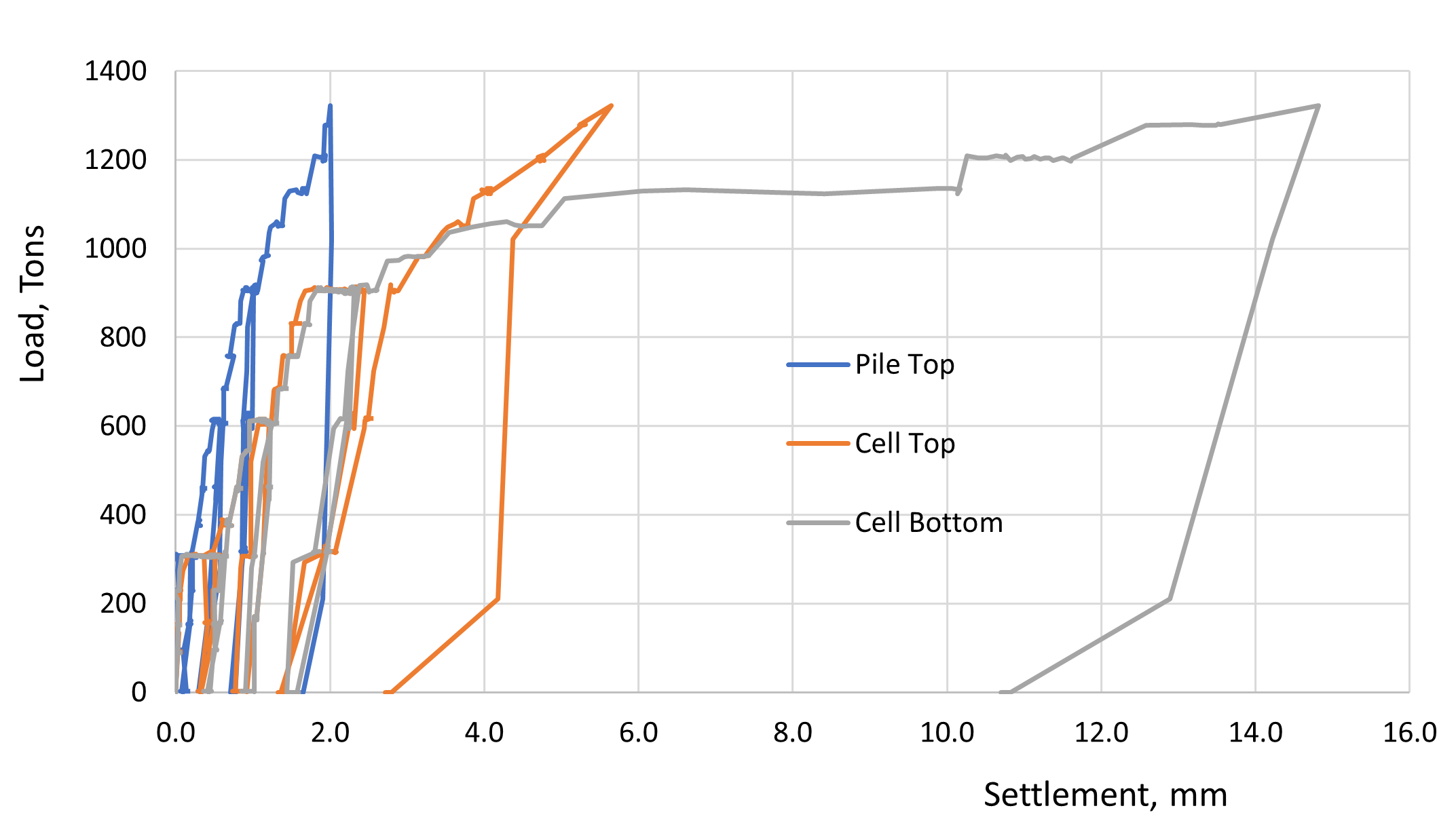
The movement at pile head and top and bottom of the cell are plotted to corresponding jack loads in Fig.5. The graphs are very interesting, and they clearly show how identical were the top and bottom piles until the load reached around 10160 kN after which the bottom pile failed and has undergone excessive settlement with very little increase in load.
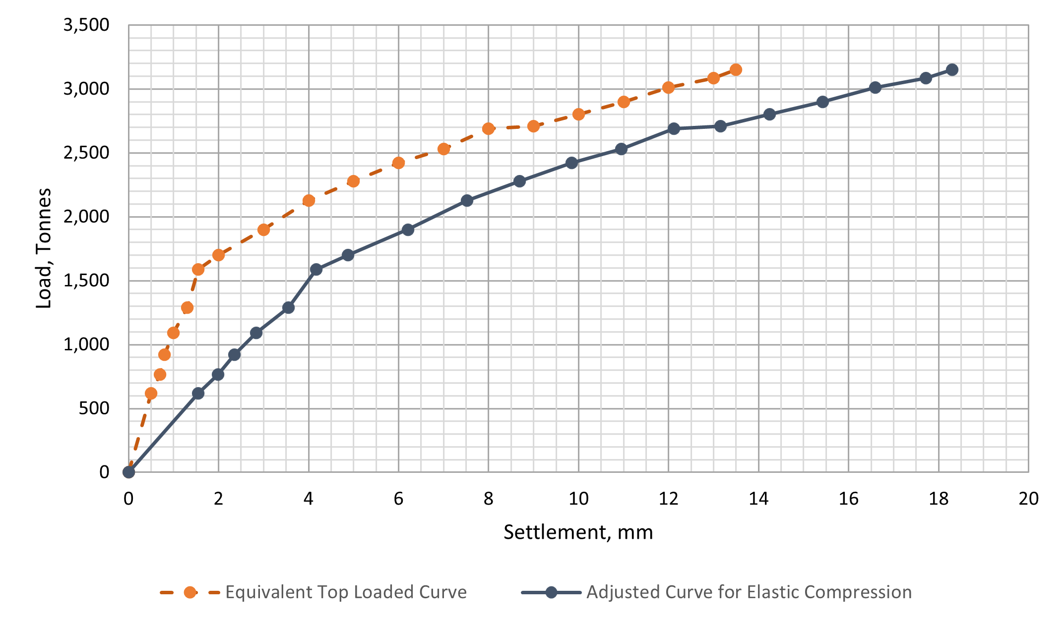
The load settlement curve of the 12m pile is constructed by a method suggested by the founder of these types of tests, Jori Osterberg. The reader may refer to Osterberg, (1995) for details. The final estimated graph is shown in Fig.6.
Adopting a suitable T-z curve for the Sandstone from the BDSLT results
Finding a suitable T-z curve to use it for a specific project is not an easy task. It needs a lot of judgment and understanding of the behavior of soil or rock pile interaction, testing circumstances, local experience, and finally needs to test the curve adequacy by comparison with field test data. As it can be seen there are several T-z curves in Fig.4.
In O-Cell tests, usually, the skin friction values adjacent to the cell are very high and do not represent an average behavior of the soil or the rock. The engineer can average the results of that segment with another segment of the pile below or above the cell. Another way to decide is to plot manually an average curve to represent the whole bunch of curves available. If the pile is not failing, the skin friction will obviously fall close to one curve but if the pile fails and passes the ultimate skin resistance the curves of the failed zone may get diverged from each other as the load transmits from the weaker zones to zones that still have stronger parts. The latter issue may be detected in Fig.4 where the curves are all close to each other in the beginning and start to deviate from each other as failure progresses in the bottom pile while the curves of the top pile are still having a trend close to each other.
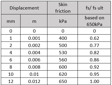
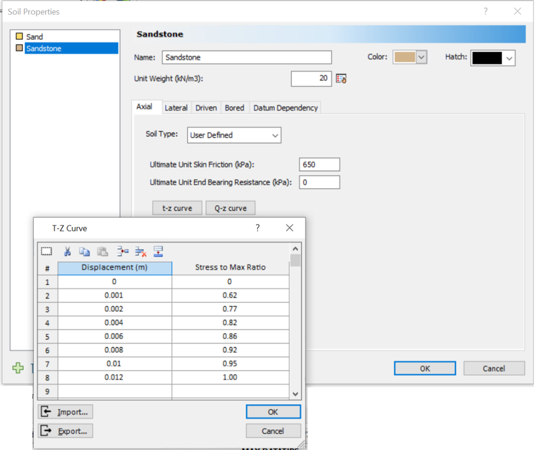
The author usually prefers to try a manually averaged curve and test the choice in a software program such as RSPile. In this study, a curve similar in shape to the curves of the bottom pile and having close ultimate skin friction close to the calculated ones with the “Bored” mode of RSPile will be adopted and it will be tested for overall behavior and adjusted if needed. The ultimate skin friction calculated with Kulhawy and Phoon method although less conservative seems to be closer to the reality at c values between 2 and 3. A value for ultimate skin friction of 650 kPa seems to be reasonable. Hence, curves of the bottom pile may be averaged near the curve of the zone SG5-SG6 where the mobilized skin friction reaches around 650 kPa at 10mm (1% of the diameter) and it lies in the sandstone range calculated previously. The curve to be used and examined may be determined with some picked points from the graph and tabulated in a ready form to apply to RSPile user-defined T-z Curve choice in Table 4. These values should be input to RSPile as shown in Fig.7. The program requires the pile section reinforcement and concrete strength as well.
Table 4: The initial T-z curve adopted for the analysis with RSPile

RSPile Results & Discussion
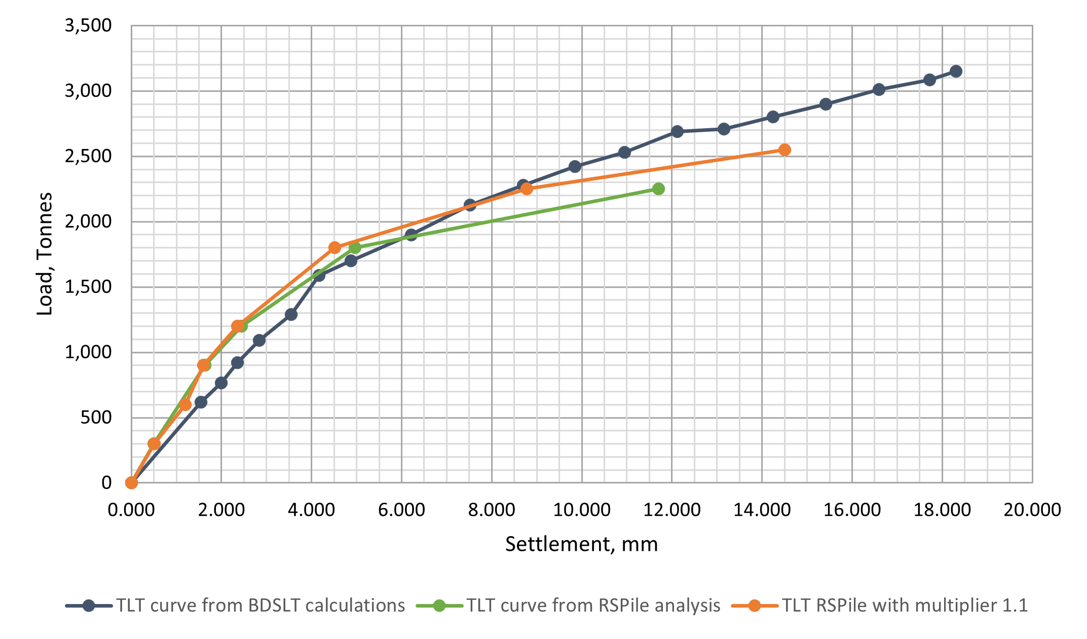
After establishing the RSPile model the pile is given a load as per the stages given in tables before. For each load you need a run and record of result settlement. The user may copy the pile as many times as he/she wants and distribute the loads on those piles and run them in one shot. Any how, the results of the program run with the given T-z curve as shown in Table 4, are plotted in Fig.8. The program did not converge at higher loads at the specified accuracy of 0.0001. A multiplier may be used to change the shape and extension of the resulting load settlement curve. The multiplier is added in the “Edit Pile” dialogue box. Atrial is shown in Fig.8 again with a multiplier of 1.1 applied to both displacement and mobilized skin friction ratio. Different multipliers may be used for displacement and load and also may be varied with depth as well.
It can be seen from Fig.8, that RSPile is an efficient tool to get the chosen T-z curve tested and the program will be ready then to analyze any pile in that sandstone with any diameter or length under any load.
--
Further Reading
Osterberg, Jorj O., (1995): “The Osterberg Cell for Load Testing Drilled Shafts & Driven Piles” Federal Highway Administration, Publication No. FHWA-SA-94-035
ASTM D8169/D8169M, (2018): Standard Test Methods for Deep Foundations Under Bi-Directional Static Axial Compressive Load”. ASTM International.
ICE Specifications for Piling and Embedded Retaining Walls, 2nd ed., 2007, Thomas Telford. The UK.
RSPile Theory Manuals, www.rocscience.com help items.