2 - Time-Dependent Consolidation

1.0 Introduction

Topics Covered in this Tutorial:

• Staging
• Groundwater
• Time-Dependent Consolidation
• Point Query
• Line Query
• Graph Query

Finished Product:

The finished product of this tutorial can be found in the Tutorial 02 Consolidation.s3z file. All tutorial files installed with Settle3 can be accessed by selecting File > Recent Folders > Tutorials Folder from the Settle3 main menu.

2.0 Model

For this tutorial we will start with the model from Tutorial 1 – Quick Start. If you have not done Tutorial 1 - Quick Start then please do so now. Alternatively, the finished product of Tutorial 1 - Quick Start can be found in the file Tutorial 01 Quick Start.s3z in the Examples > Tutorials folder in the Settle3 installation folder.

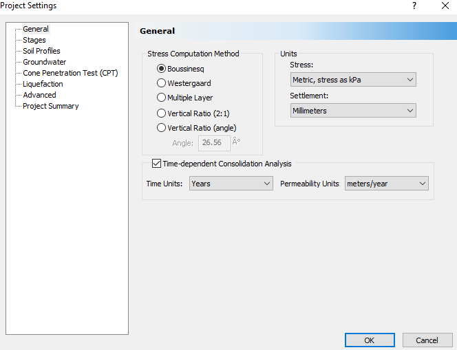
2.1 Project Settings

1. Open by selecting Home > Project Settings
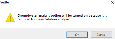
2. Under the General tab, select the Time-dependent Consolidation Analysis checkbox. You will see a warning that the Groundwater analysis option will be turned on:



3. Click OK.
4. Set the Time Units = Years, and the Permeability Units = meters/year. The dialog should look like this:



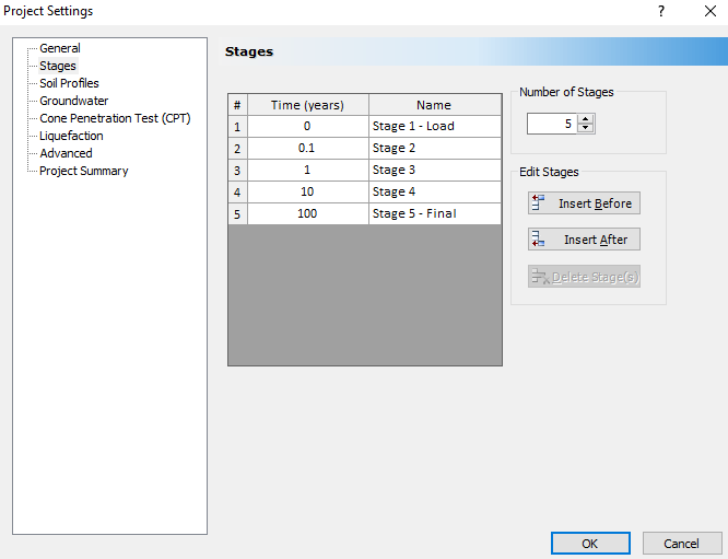
5. Click on the Stages tab. Stages in Settle3 can represent:
• different times at which you wish to view results (for a consolidation analysis), and/or,
• additions or changes to the model input parameters (e.g. added or modified loads).
6. Set the Number of Stages = 5, and assign times and names to these stages as shown below.



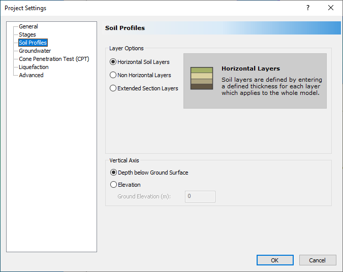
7. Select Soil Profiles tab. Select 'Depth below Ground Surface'.



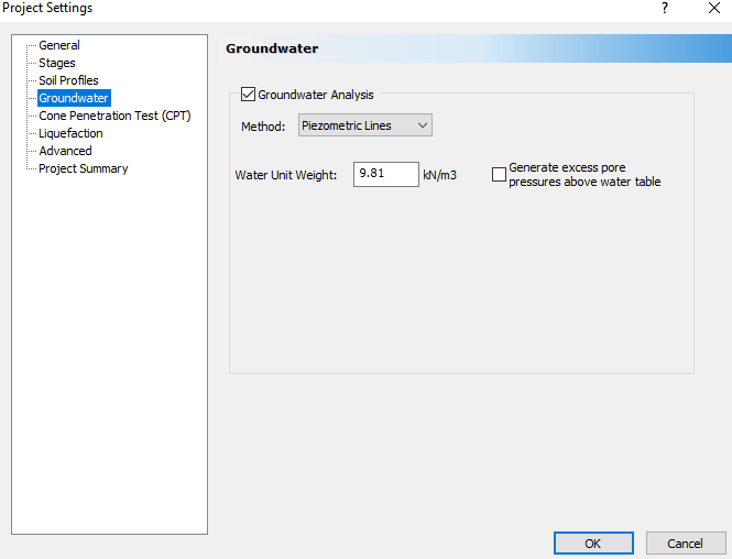
8. Click on the Groundwater tab. Here you can set the unit weight of water. Leave the default values.



9. Click OK to save the changes and exit the dialog.

2.2 Assign Piezometric Line

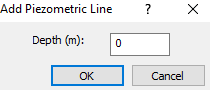
1. Select Groundwater > Add Piezometric Line
2. In the dialog that pops up, you can set the depth of the water table. Recall that 0 m is the ground surface. Leave the default value of 0m as this will define a water table which is at the ground surface.



3. Click OK to close the dialog.
4. The Assign Piezometric Line to Soils dialog will appear. Click on the checkbox beside Medium Clay, and select OK. This will assign the water table to ONLY that material for all stages.

2.3 Soil Properties

For time-dependent consolidation, we need to assign additional material properties.

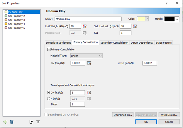
1. Select Soils > Define Soil Properties
2. Go to the Primary Consolidation tab and under Time-dependent Consolidation Analysis set Cv to 3. The Cv parameter is the coefficient of consolidation, which influences the time it takes for excess pore pressure to dissipate. Leave all other parameters so that the dialog looks like this:



3. Click OK to close the dialog.

2.4 Soil Layers - Drainage

In Tutorial 1 we set the layer thicknesses. Now we will discuss the drainage conditions.

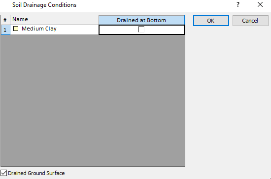
1. Select Soils > Layers
2. Click on the Drainage Conditions button, located at the top right hand corner of the dialog, and you will see the Soil Drainage Conditions dialog as shown.



3. Notice the Drained Ground Surface checkbox at the lower left corner of the dialog. If this checkbox is selected it means that the pore water pressure at the Ground Surface is 0 and water is free to flow out of the soil. Make sure the Drained Ground Surface checkbox is checked.
4. We will assume that water cannot flow out of the bottom of the clay layer (the clay is underlain by impermeable bedrock), so leave the Drained at Bottom checkbox next to the Clay layer unchecked.
5. Click OK twice to close both dialogs.

3.0 Computation and Results Visualization

By default, query results are automatically re-computed after editing input data, however, the field point grid results are NOT automatically re-computed. (These settings can be configured in the Autocompute dialog in the Analysis menu).

To re-compute results for the field point grid, line query and point query:

1. Select Results > Compute

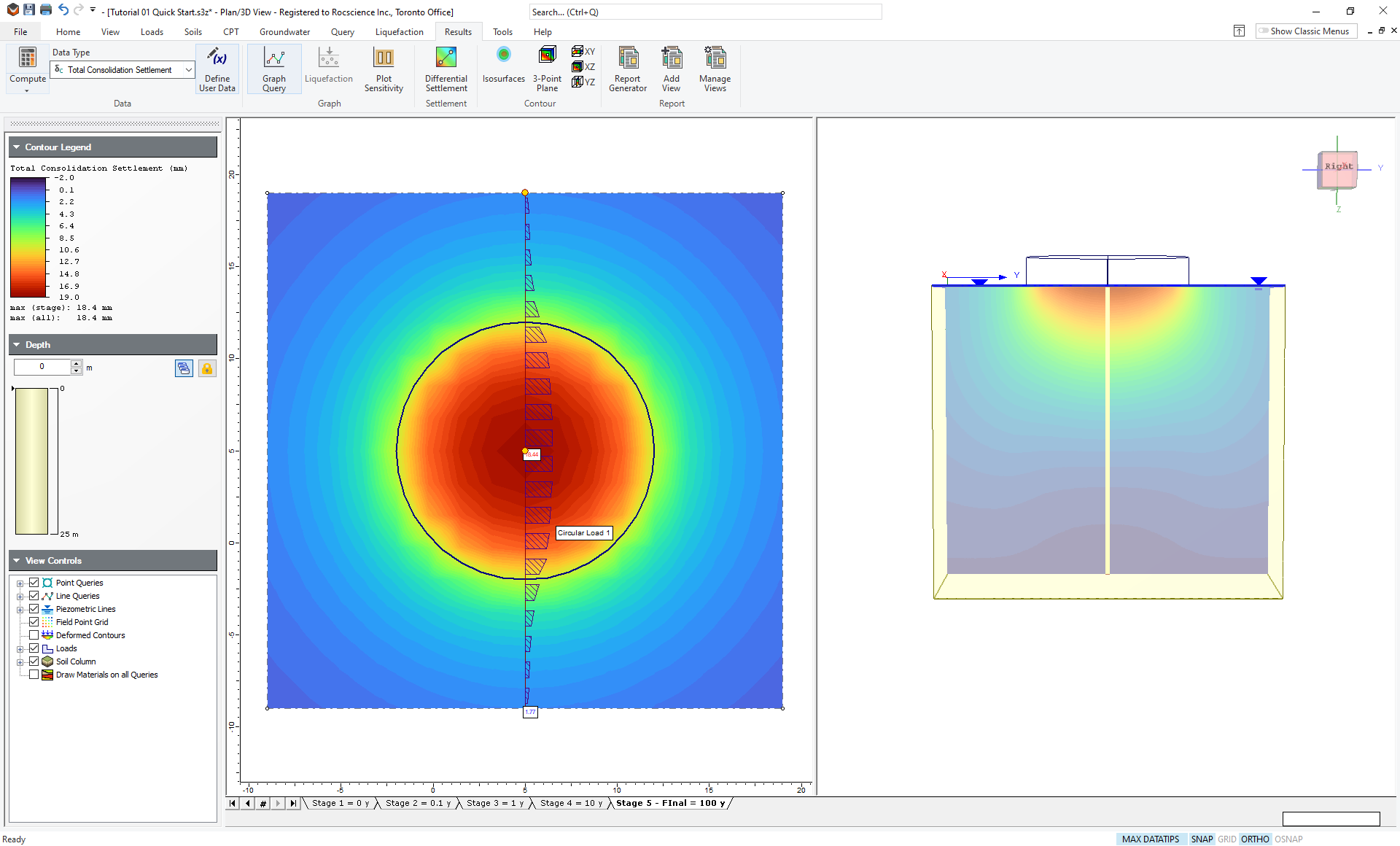
3.1 Total Settlement

By default, contours for the Total Settlement will be shown.

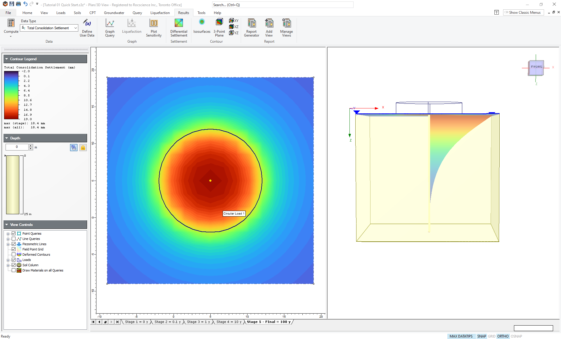
1. In the Results tab and change the plot to 'Total Consolidation Settlement' using the drop-list of data types at the top of the screen.
   
   If you are looking at Stage 1, you will see that there is no consolidation settlement. This is because when the load is applied, all of the stress is accommodated by an increase in pore pressure. There is no consolidation settlement until some time passes and pore pressures dissipate transferring stresses to the soil matrix causing displacement.
   
2. Click through the other stages and you will see increasing consolidation settlement with time. The contours for Stage 5 - Final (100 years) should look like this:

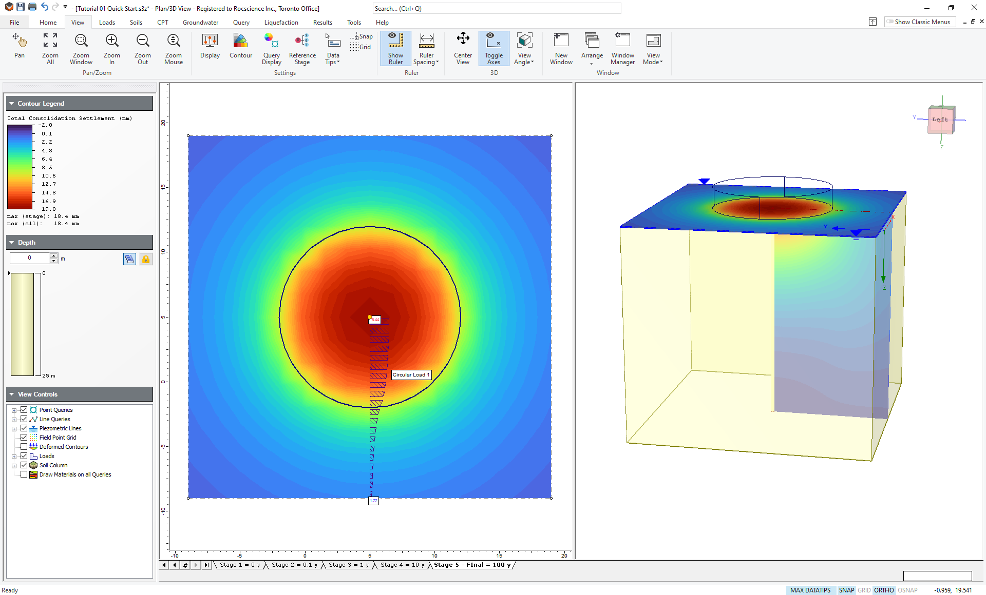
The maximum consolidation settlement at Stage 5 is 18.4 mm as indicated below the contour legend in the sidebar.

4.0 Queries

To obtain results at specific locations, you can add Query Points or Query Lines. These allow you to graphically plot data versus depth or horizontal distance, as discussed in the Tutorial 1 - Quick Start.

From the previous tutorial, you should have one Query Point and one Query Line still defined. Let’s first look at the Query Point results.

1. Ensure that you are plotting Total Consolidation Settlement and that you are looking at Stage 5 – Final. Rotate the model in the 3D View so that the screen looks as follows:

In the 3D View you can see the Consolidation Settlement plotted along the vertical line represented by the query point.

4.1 Excess Pore Pressure

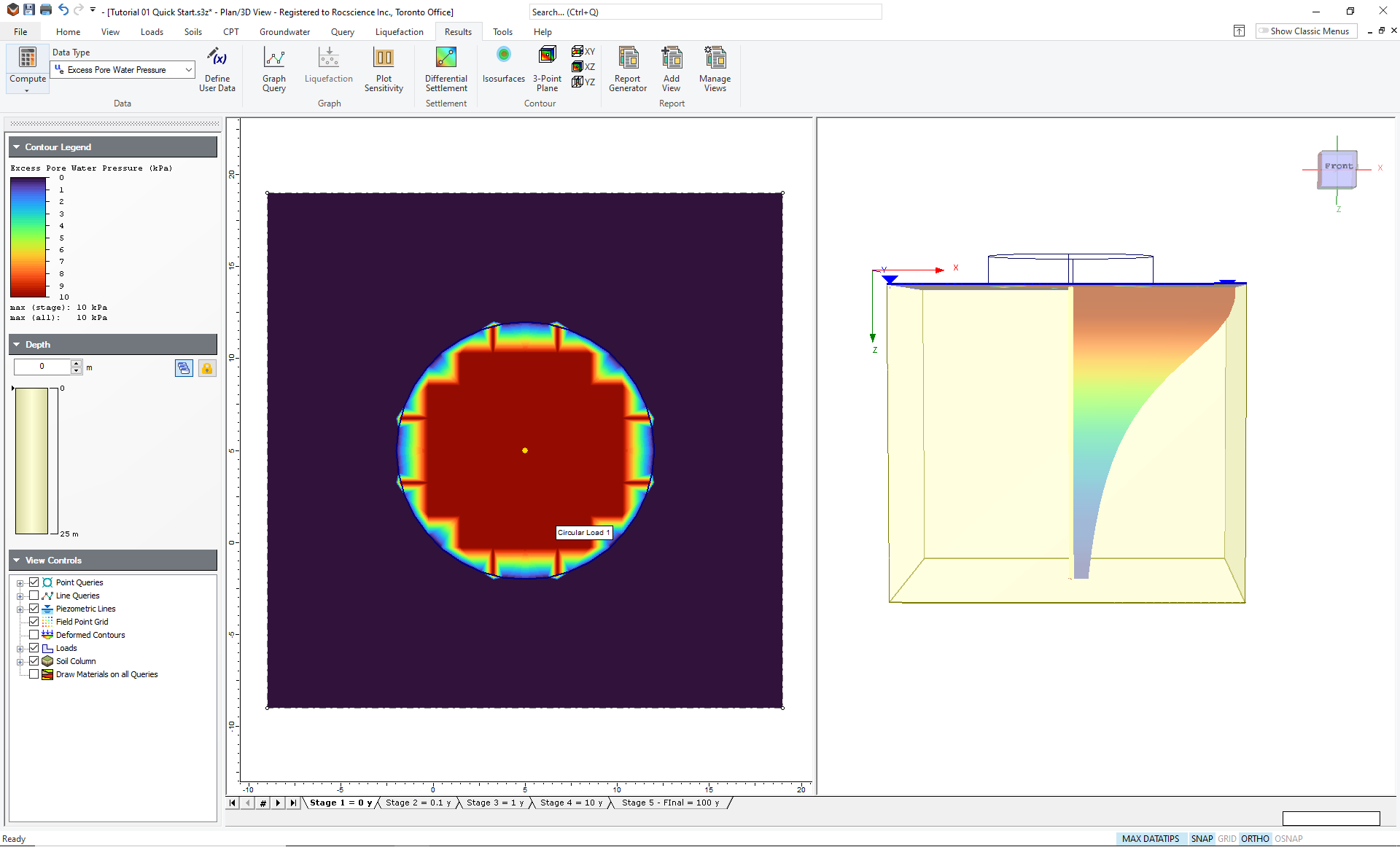
1. Use the data type dropdown menu to change the data being plotted to Excess Pore Water Pressure.
2. Go back to Stage 1 and your screen should look like this:



3. Click through the stages and you can see how the pore pressure dissipates with time.
   

Now let’s graph the Query Point Data. In order to select the Query Point for graphing, we will have to first delete or hide the Query Line, because it overlaps the Query Point.

1. Go to the View Controls in the Sidebar, and turn off the Line Queries checkbox. The Query Line is now hidden.
2. Now right-click on the Query Point in the Plan View, and select Graph Query from the popup menu. You will see a dialog asking what you wish to plot.
3. Choose Excess Pore Water Pressure.
4. At the bottom of the dialog hit the Select All button to choose all stages for plotting. The dialog should look as follows:
   
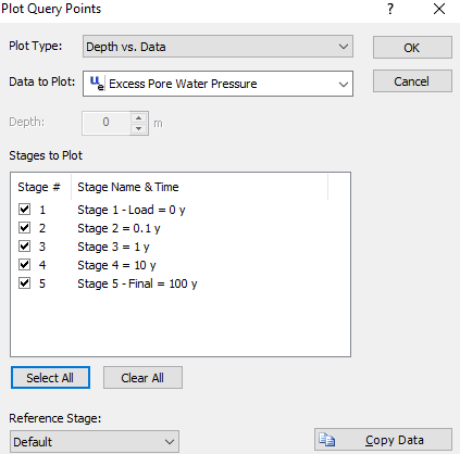
5. Click OK to generate the graph.
   

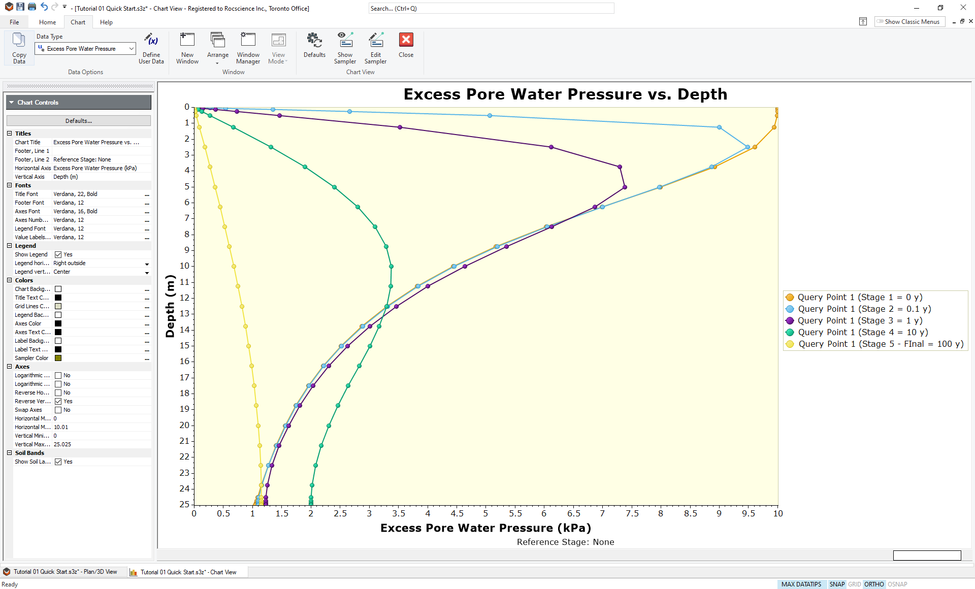
Here you can see the excess pore water pressure plotted versus depth at different times. You can see the pore pressure generally decreasing with time. You can also see how the bulb of high pressure that starts at the surface moves downwards as water flows from areas of high pressure to areas of lower pressure.

4.2 Effective Stress

1. Still looking at the graph, change the data type to Effective Stress ZZ.



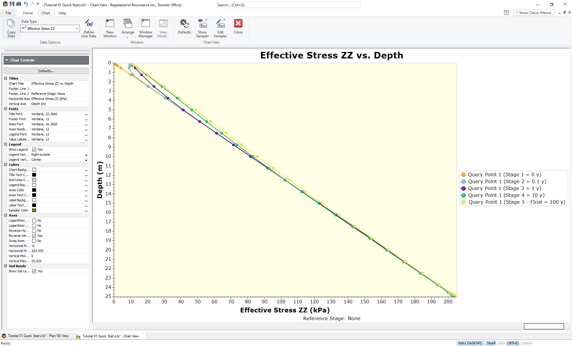
The stress generally increases with depth due to gravitational loading. However you can see how the effective stress near the surface increases with time as the pore pressure dissipates.

2. Close the graph view.

4.3 Line Query

1. Go to the View Controls in the Sidebar, and select the Line Queries checkbox to re-display the Query Line.
2. Change the data type to Total Consolidation Settlement.
3. Right-click on the starting point of the query line (at the center of the load), and select Move To from the popup menu.
4. Enter the point (5,19) in the prompt line, to extend the query line across the entire load.
5. Go to Stage 5 and rotate the model in the 3D View so that screen looks as follows:



6. Select the stage tabs 1 through 5, to view the increase in consolidation settlement with time, in the 3D View.
7. Change the data type to Excess Pore Water Pressure.
8. Select the stage tabs 1 through 5, to view the decrease in excess pore pressure with time, in the 3D View.

This concludes the Time-Dependent Consolidation tutorial; you may now exit the Settle3 program.