3 - Storage Tank on Embankment

1.0 Introduction

Topics Covered in this Tutorial:

• Load Staging
• Embankments
• Multiple Materials
• Time-Dependent Consolidation Analysis
• Immediate and Consolidation Settlement

Finished Product:

The finished product of this tutorial can be found in the Tutorial 03 Storage Tank.s3z file. All tutorial files installed with Settle3 can be accessed by selecting File > Recent Folders > Tutorials Folder from the Settle3 main menu.

2.0 Model

If you have not already done so, run Settle3 by double-clicking on the Settle3 icon in your installation folder. Or from the Start menu, select Programs > Rocscience > Settle3.

2.1 Project Settings

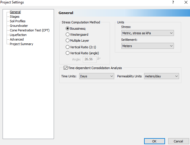
1. Select Home > Project Settings to open the Project Settings dialog and make sure the General tab is selected.
2. Define the Stress units = Metric, stress as kPa.
3. Set the Settlement units = Meters.
4. Select the Time-dependent consolidation analysis checkbox.
5. Set the Time Units = Days, and the Permeability Units = meters/day.
6. A message will appear informing you that the groundwater analysis option will be turned on because it is required for consolidation analysis. Click OK.



7. Click on the Stages tab and set the Number of Stages = 13. Fill in the stage times as shown:

8. Select Soil Profile tab, select 'Depth below Ground surface'.

   

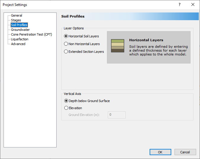
9. Click OK to close the Project Settings dialog.

10. Select Home > Project Summary and enter “Storage Tank Tutorial” as the project title. Click OK to exit the dialog.

3.0 Assign Piezometric Line

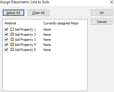
1. Select Groundwater > Add Piezometric Line
2. Set the Depth to Water table = 2 m.
3. In the Assign Piezometric Line to Soils dialog, click on Select All to assign groundwater to every soil layer in the model.

4.0 Adding the Embankment

1. Select Loads > Loads by Layers to open the Embankment Designer dialog.
2. In the Embankment Designer dialog, enter Base Width = 200 m and both the Near End Angle and Far End Angle = 8 degrees.
3. Now change both the Left Angle and Right Angle to 8 degrees.
4. Change the Height to 7 m. Leave all other parameters with the default values.
   
   Your dialog should look like this: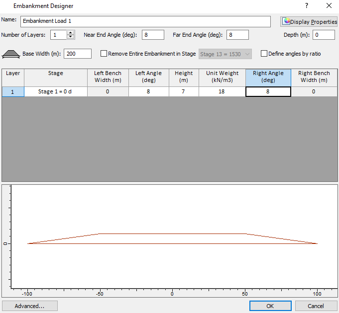
   
5. Click OK. You will see crosshairs and will be prompted to pick the near point of the embankment centerline. You can use the mouse to click on the Plan View or manually enter the coordinates.
6. Enter {0,-125} then press Enter.
7. Now you will be prompted to pick the far point of the embankment centerline. Enter {0,125} and press Enter.

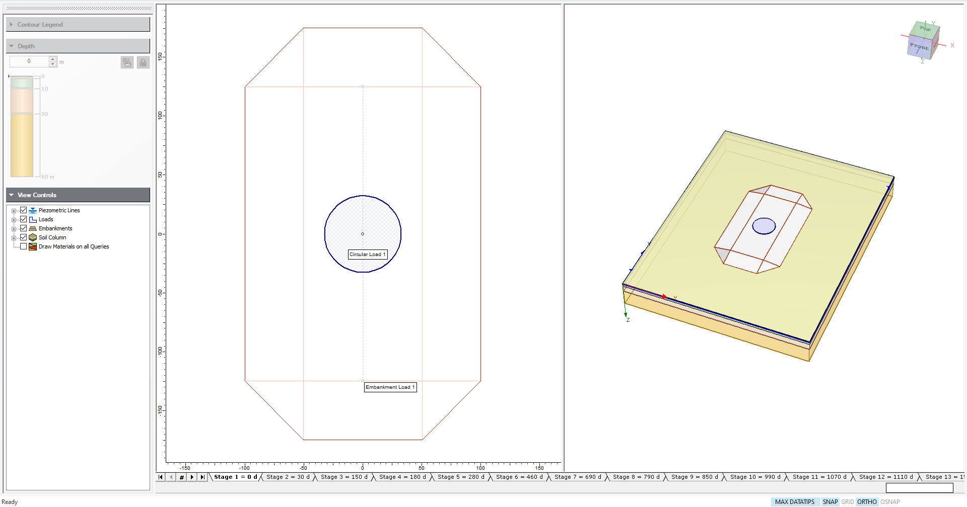
You should now see the embankment both in the Plan View (left) and in the 3D View (right). If the embankment is not visible in the Plan View, click in the Plan View and select Zoom All or press the F2 function key.

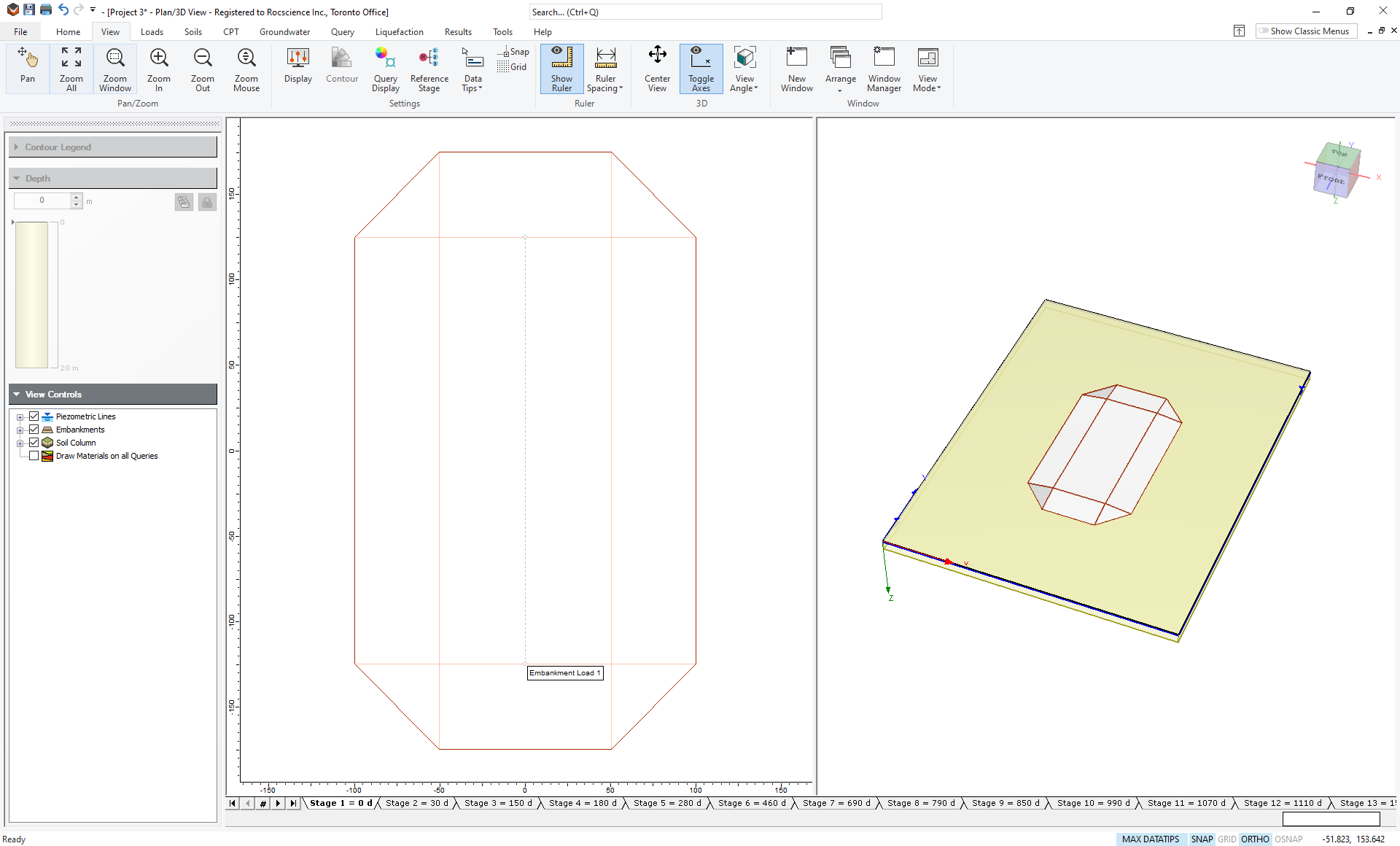
5.0 Adding the Load

The storage tank will be modelled by a circular load.

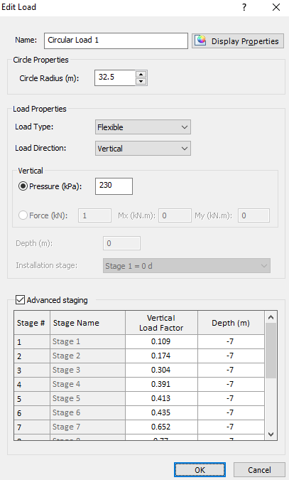
1. Select Loads > Circular Load
2. Change the Circle Radius to 32.5 m with a Pressure of 230 kPa.
3. Since the loading will be changing with each stage, check the Advanced staging box and enter the data given in the table below.

Stage #	Vertical Load Factor	Bottom Depth (m)
1	0.109	-7
2	0.174	-7
3	0.304	-7
4	0.391	-7
5	0.413	-7
6	0.435	-7
7	0.652	-7
8	0.770	-7
9	0.870	-7
10	0.943	-7
11	0.962	-7
12	1	-7
13	1	-7



4. Click OK.
5. You will now see a circle that needs to be placed somewhere on the Plan View. You can click the mouse to place the circular load, or alternatively, you can enter the coordinates in the prompt line at the bottom right of the screen.
6. Enter {0,0} and hit Enter to place the center of the circular load at the center of the embankment.

You should now see the embankment and the circular load in both the Plan View (left) and 3D View (right). Look through the various stages by selecting the tabs at the bottom of the screen. The circular load should be changing (increasing in height) as you go through the various stages.

6.0 Soils

6.1 Soil Properties

1. Select Soils > Define Soil Properties
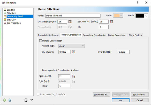
2. For each of the first three materials, turn on Immediate Settlement and change the Primary Consolidation Material Type to Linear.
3. Enter data for the first three soil types as shown:

Soil Property Field	Name	Es (kPa)	Esur (kPa)	Cv (m2/day)
Soil Property 1	Sand Fill	25000	25000	0.25
Soil Property 2	Silty Sand	20000	20000	0.25
Soil Property 3	Dense Silty Sand	25000	25000	2.0

4. Leave all other properties at their default values. The dialog for Soil Property 3 should look like this:



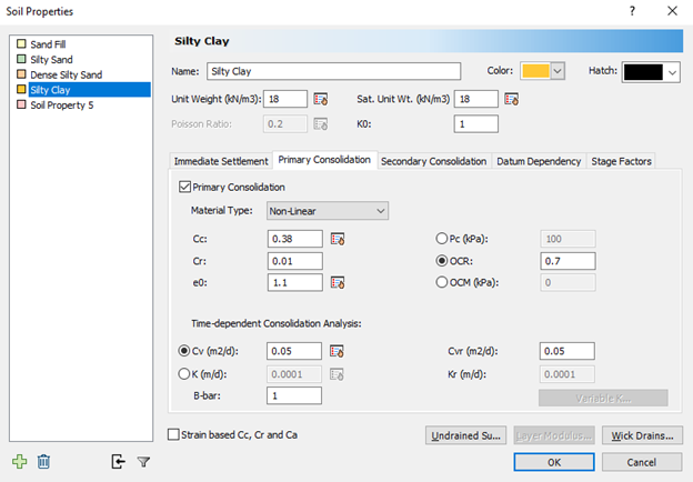
5. For Soil Property 4, turn on Immediate Settlement and change the Primary Consolidation Material Type to Non-Linear. Enter the following parameters:

Your dialog should look like this:

6.2 Soil Layers

To define the thickness of the soil layers:

1. Select Soils > Layers
   Here you can add layers of different materials and change their thickness.
2. Click the Insert Layer Below button three times, to create a total of four layers. By default, the material types are assigned in the same order as they are defined in the Soil Properties dialog. We will use the default assignments. You can change material assignments by clicking on the Name and selecting a material type for the layer.
3. Define the thickness for each layer as shown below:
   • Sand Fill = 2
   • Silty Sand = 8
   • Dense Silty Sand = 20
   • Silty Clay = 50
   
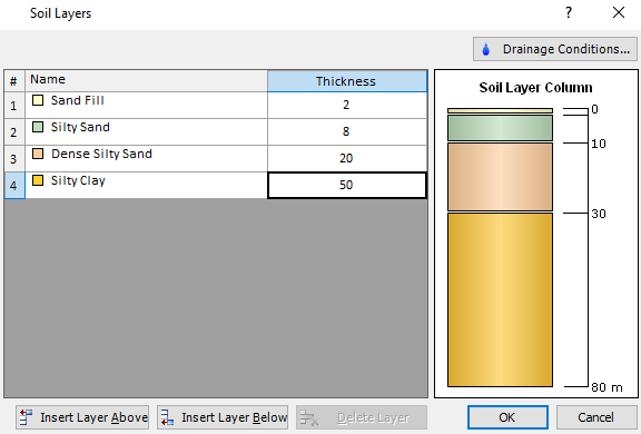
4. Click on the Drainage Conditions button. Check the Drained at Bottom checkbox for the Silty Clay and for the Dense Silty Sand.
   
   
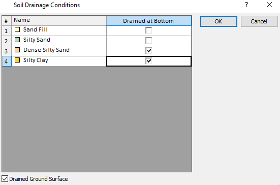
5. Click OK twice to close both dialogs. The model should appear as follows:
   

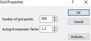
7.0 Field Point Grid

1. Select Query > Auto Field (Point Grid)
2. Enter Number of grid points = 500 and Autogrid expansion factor = 1.2.
3. Select OK.

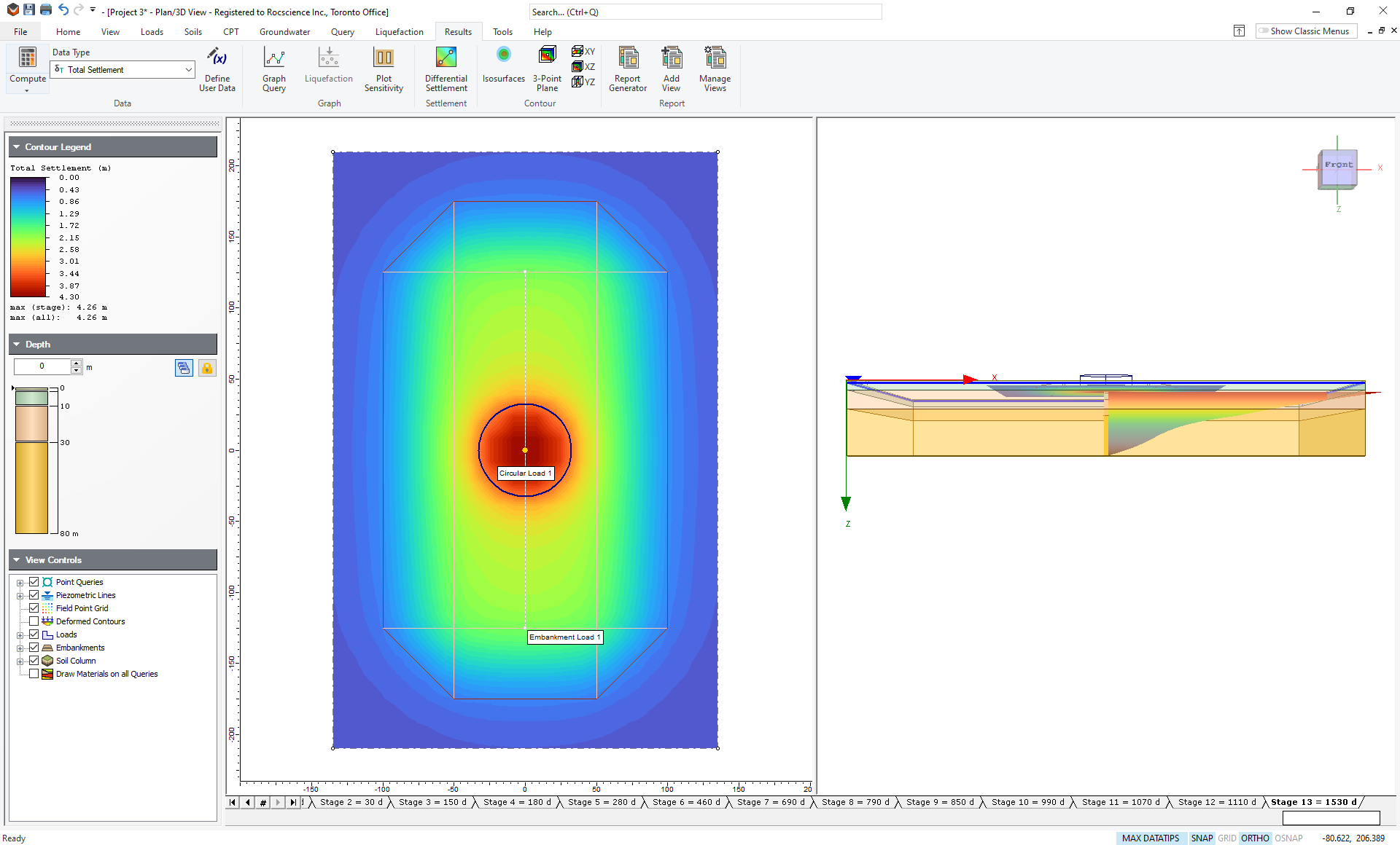
A grid will be generated while the stresses and settlements will be automatically calculated throughout the 3-dimensional volume. This will take a little time, depending on the speed of your computer. By default, contours of Total Settlement will be shown (as shown in the Results tab). Select the final (Stage 13) tab and you should see the following results.

TIP: If you wish to view the location of the field points, go to View > Query Display Options and under Field Point Grid, choose a symbol other than None.

8.0 Results Visualization

8.1 Total Settlement

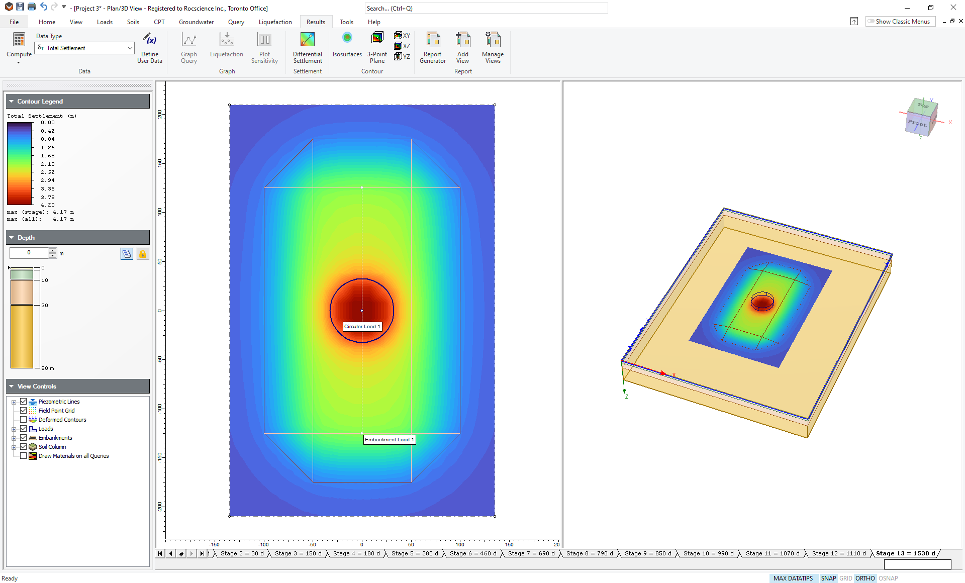
You should be looking at the contours of total settlement in the Plan View and the 3D View. Under the Contour Legend in the Sidebar, you can see that the maximum settlement is 4.17 m. You can visualize this displacement in the 3D View by clicking on View Controls in the Sidebar and turning on the checkbox beside Deformed Contours. Rotate the 3D View (hold down the left mouse button and move the mouse) so that you can view the deformed settlement as shown below.

TIP: The deformation of the surface is exaggerated. The scale factor can be changed in the Query Display Options dialog (View > Query Display Options > Field Point Grid > 3D View).

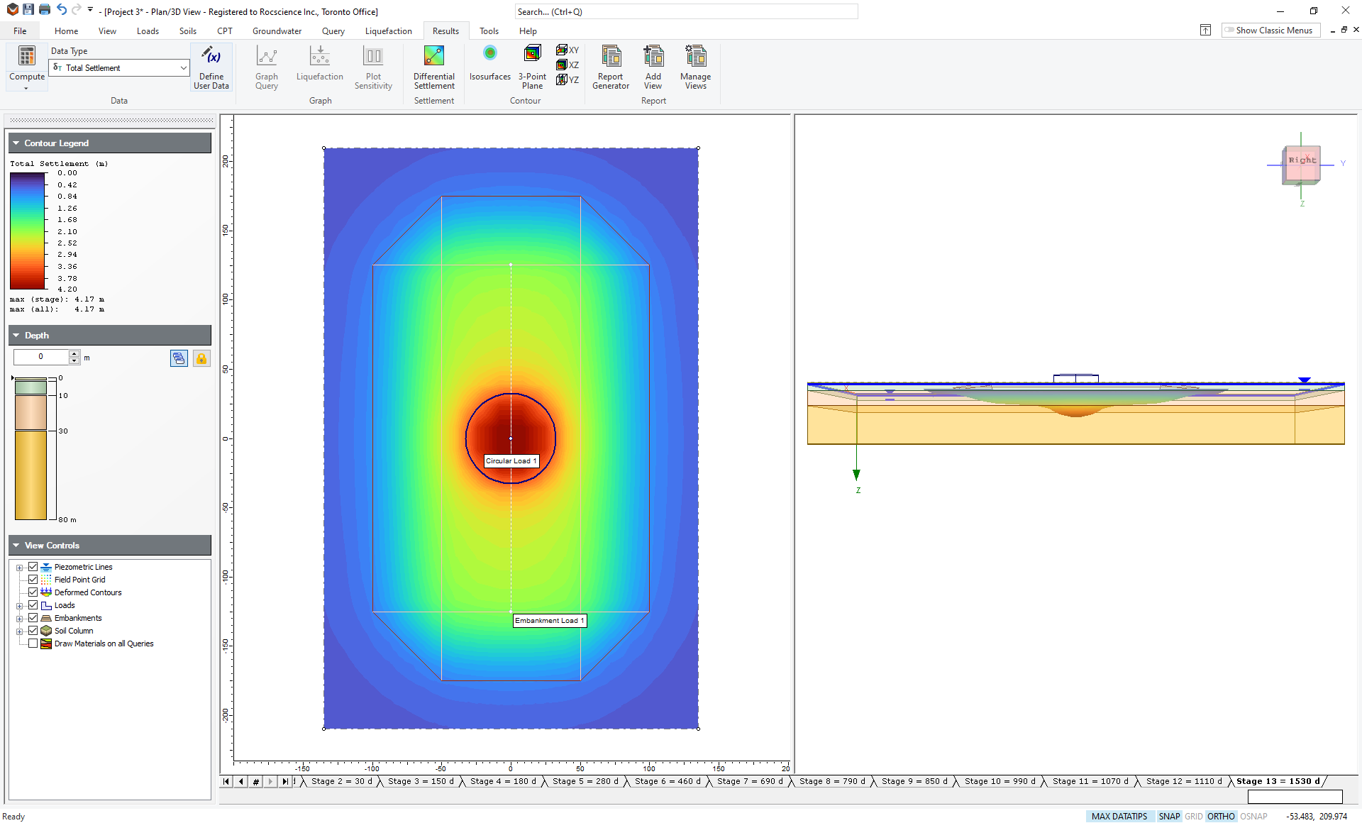
By default, the settlement at the ground surface (Depth = 0) is shown. You can examine the settlement at different depths by using the depth control in the Sidebar. The Settlement at a depth of 15 m looks like this:

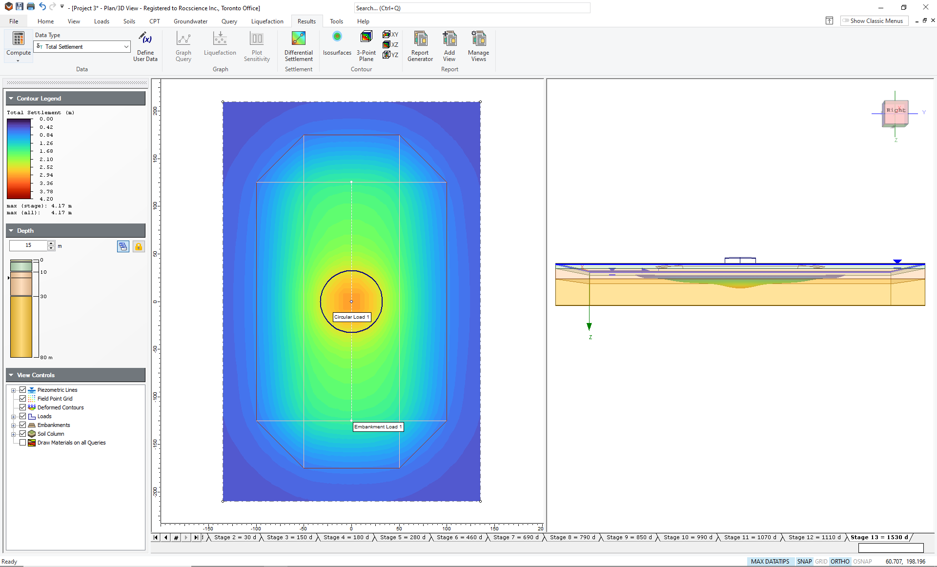
TIP: You can change the contour range, interval and color scheme by choosing Contour Options from the View menu.

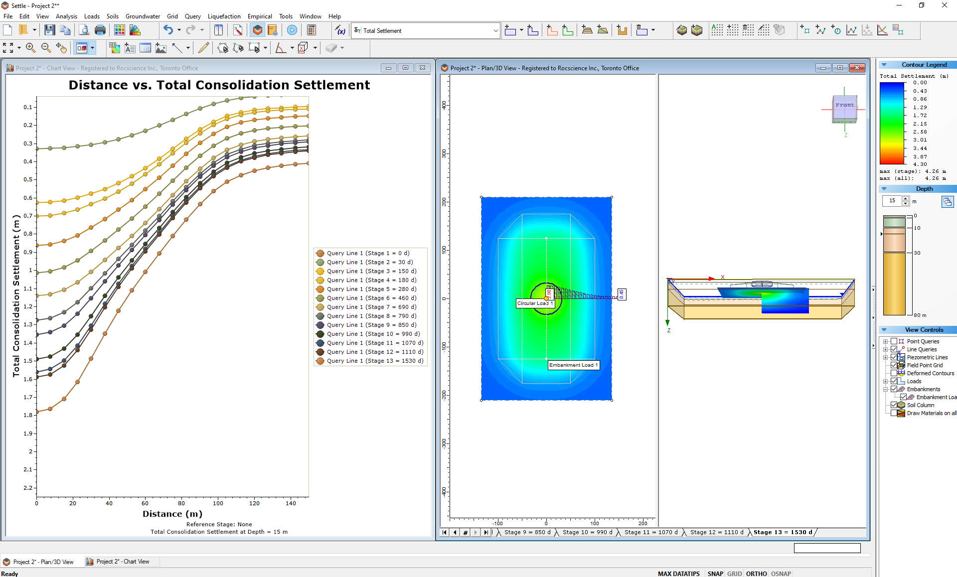
8.2 Plotting Other Data Types

On the toolbar at the top, you can change the data type being plotted. As well as Total Settlement you can select Immediate Settlement or Total Consolidation Settlement. The Total Settlement is the sum of the Immediate Settlement and Consolidation Settlement. Therefore plotting either one of these will show less displacement than the Total Settlement. In this case, the maximum Immediate Settlement is 1.4 m and the maximum Consolidation Settlement is 2.78 m.

You can also plot the Loading Stress or Total Stress. The Loading stress is simply the stress due to the load, whereas the Total Stress is the Loading Stress plus the stress due to gravity and the hydrostatic pressure from the groundwater (i.e. self-weight of the soil).

8.3 Queries

To obtain results at specific locations, you can add Query Points or Query Lines. These allow you to graphically plot data versus depth, horizontal distance, or time at any location in the model.

8.3.1 Query Points

1. Select Query > Add Point
   You will see the Query Point dialog as shown.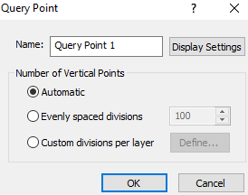
   
2. Leave the default choice of Automatic. This will generate subdivisions such that the discretization is denser near the ground surface and at layer boundaries, where the high-stress gradients are likely to be.
3. Click OK and the cursor will become a cross-hairs in the Plan View.
4. You now need to specify the location of the Query Point on the surface. Click on the point at the center of the circular load.
5. Change the plot type back to Total Settlement, turn off the deformed contours and set the viewing depth back to 0 m. Rotate the model so that you can view the point query results in the 3D View as shown below.

The Total Settlement is plotted along the vertical line represented by the query point.

To graph this data:

1. Select Results > Graph Query
2. Select the Query Point using the mouse and hit Enter.
   
   TIP: A shortcut to graph query data is to right-click on the Query Point in the Plan View, and select Graph Query from the popup menu.
   
3. In the Plot Query Points dialog, choose Data vs. Stage Time for the Plot Type, and choose Total Settlement if it is not already selected.
   
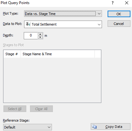
4. Select OK and you should see the following graph of Time versus Total Settlement at depth = 0.
5. In the Sidebar under Axes, change the horizontal and vertical values to the following:
   

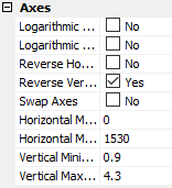
Your plot should look like this:

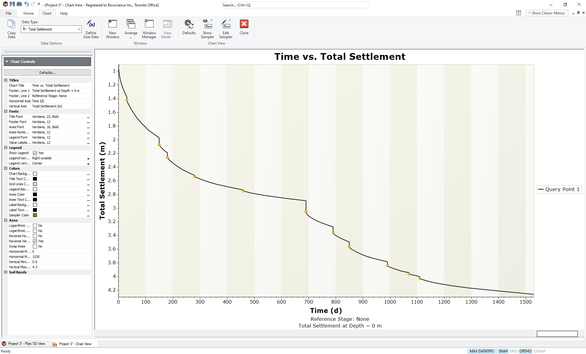
As expected, the amount of settlement increases with time as more load is applied, and the clay layer consolidates further.

8.3.2 Query Lines

1. Toggle back to the model view by clicking the Plan/3D View tab at the bottom left of the screen.
2. Select Query > Add Line
3. You are first prompted for the number of horizontal divisions. Leave the default value of 20. As with a Query Point, you are also prompted for the number of vertical divisions. This time select Evenly Spaced Divisions and change the number to 30.
   
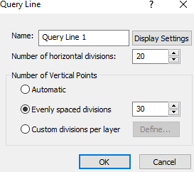
4. This will generate 20 vertical strings with 30 divisions in each string. Click OK and you will now be prompted for the start point of the line.
5. With the mouse, select the existing query point at the center of the circle.
6. You will now be prompted to enter the second point. Using the keyboard, enter the coordinates {150,0}. Hit Enter.
   
   The Query line will appear on the Plan View with bars giving the Total Settlement along the line. The minimum and maximum values are shown numerically. The 3D View will show a vertical cross-section with contours of Total Settlement. To see this clearly, turn off the Point Query by clearing the checkbox next to Point Queries on the Sidebar (under View Controls). Your screen should now look like this: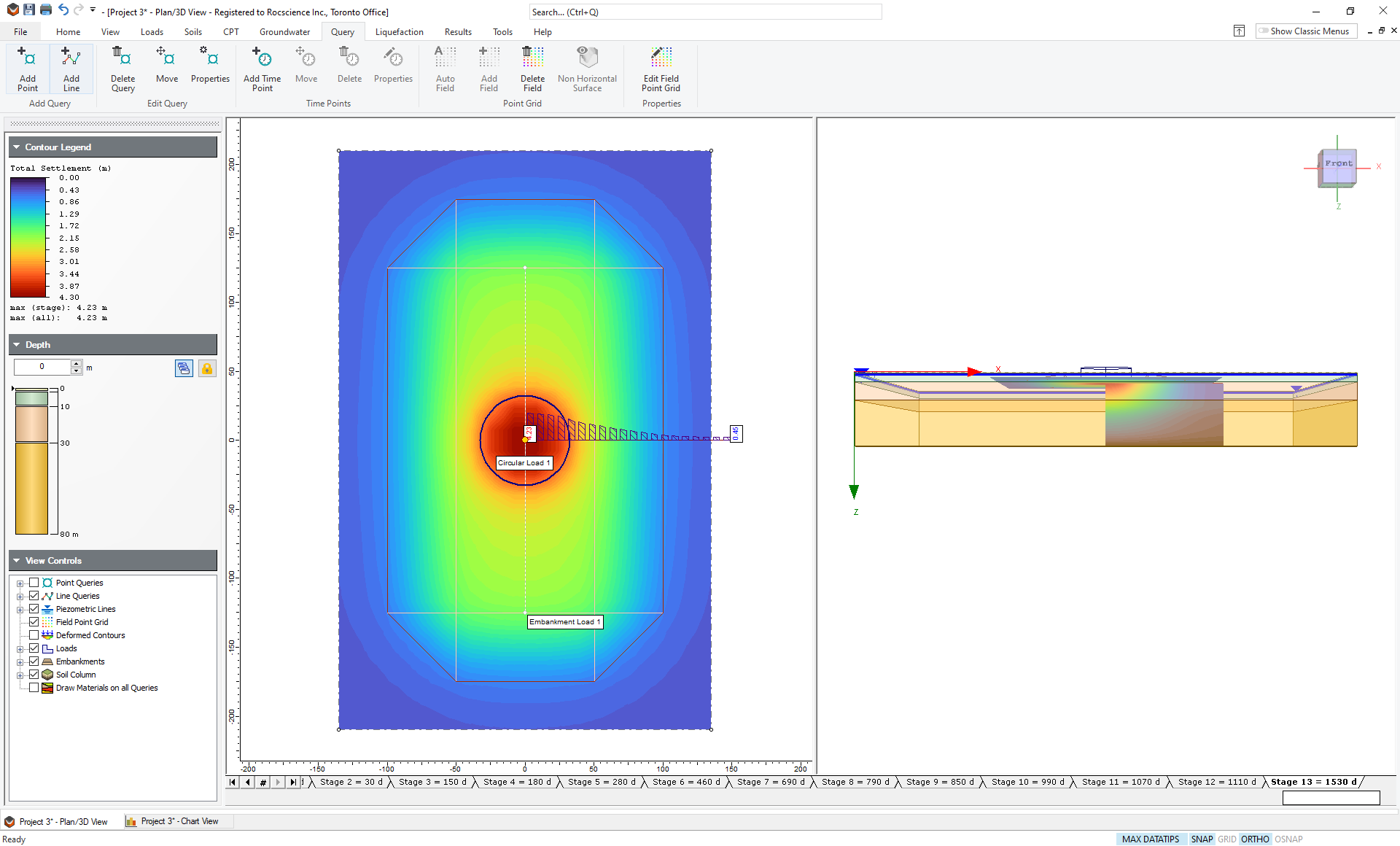
   
7. You can now plot the data by selecting Results > Graph Query and selecting the line (or by right-clicking on the line and choosing Graph Query).
8. Choose Total Settlement as Data to Plot and Select All for Stages to Plot.
   
   
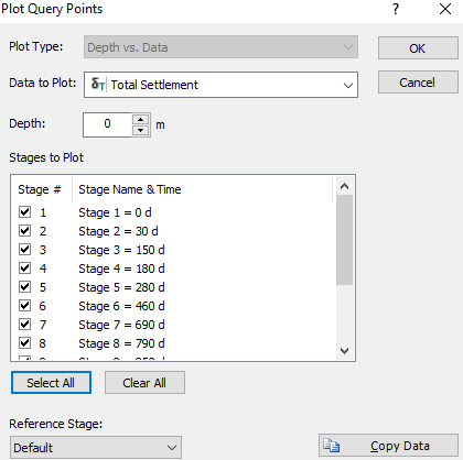
9. You will now see a graph showing the Total Settlement versus horizontal distance along the line at all 13 stages. In the Sidebar under Axes, change the horizontal and vertical values to the following:
   
   
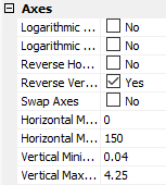
   You should see the following plot: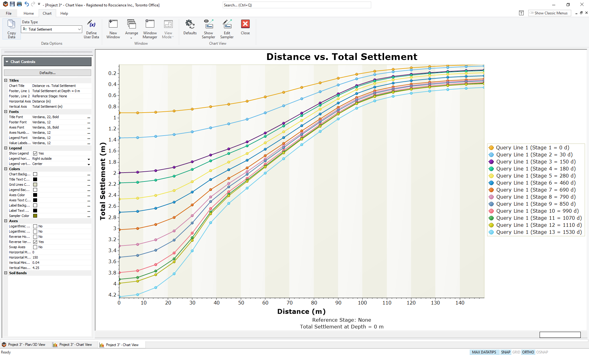
   
   
10. This is the Total Settlement along a line at the ground surface. Tile the windows so that you see both the Plan View and the Chart View.
    
11. Select Chart > Arrange > Tile Windows Vertically

You can now change the depth of the line by using the depth control in the Sidebar of the Plan view. You can also change the data being plotted using the pull-down menu at the top.

TIP: You can export this data to a Microsoft Excel spreadsheet by simply right-clicking on the graph and choosing Plot in Excel. If you prefer another spreadsheet program, then choose Copy Data and you will be able to paste it into any Windows program.

This concludes the Storage Tank tutorial; you may now exit the Settle3 program.