1 - Quick Start Tutorial

This tutorial is a simple introductory tutorial that aims to help the user become familiar with the basic modelling and data interpretation features of Settle3. Settle3 is a three-dimensional program for the analysis of vertical consolidation and settlement under foundations, embankments and surface loads. The program combines the simplicity of one-dimensional analysis with the power and visualization capabilities of more sophisticated three-dimensional programs.

Topics Covered in this Tutorial:

• Applying a Circular Load
• Immediate Settlement
• Primary Consolidation Settlement
• Deformed Contours
• Query Points and Query Lines
• Graph Query
• Info Viewer
• Drawing Tools

Finished Product:

The finished product of this tutorial can be found in the Tutorial 01 Quick Start.s3z file. All tutorial files installed with Settle3 can be accessed by selecting File > Recent Folders > Tutorials Folder from the Settle3 main menu.

1.0 Introduction

Before we start the tutorial, you should be familiar with the following general information about Settle3.

Program Assumptions

There are several important assumptions and limitations that must be considered when using Settle3:

• Settle3 calculates three-dimensional stresses due to surface loads. However, strain and pore pressures are computed in one-dimension, assuming only vertical displacements can occur. This is in keeping with general geotechnical engineering practice and material parameters are specified to reflect the one-dimensional nature of the analysis.

• In the Horizontal Soil Layers mode, all soil layers are assumed to be horizontal and continuous. It is not possible to specify non-horizontal soil geometry. In the Multiple Boreholes mode, non-horizontal soil strata can be defined. The ground surface is assumed to be horizontal by default, but can be modelled non-horizontal by selecting the Non-Horizontal Ground Surface option.

• By default, applied loads are flexible, so that the stress at the surface directly below the load is constant, but the displacement is not. Rigid loading can also be specified but is more limited in application.

• The default ground surface is at elevation= 0, elevation is positive upwards, and compressive stress is positive.

Program Interface

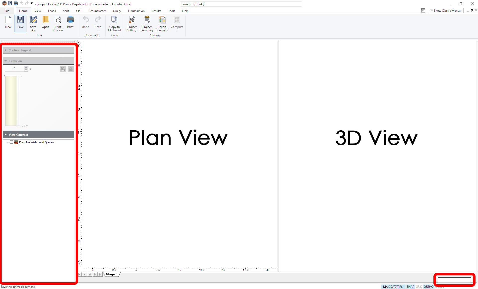
In order to carry out the various modelling and interpretation tasks, Settle3 provides two distinct views:

• The Plan View is a top-down view of the ground surface and is used to define load geometries, queries, drawing tools etc.

• The 3D View enables easy visualization of results in three dimensions.

In addition, the Sidebar at the left of the screen provides a variety of viewing controls and the contour legend. In general, both views and the sidebar are visible, but their relative sizes can be scaled as desired. Lastly, the Prompt Line at the bottom right-hand side of the screen provides the ability to enter coordinates instead of using the mouse to define the geometry of different aspects of the model (loads, preloads, ground improvement regions, etc.)

2.0 Model

If you have not already done so, run Settle3 by double-clicking on the Settle3 icon in your installation folder. Or from the Start menu, select Programs > Rocscience > Settle3.

2.1 Project Settings

The Project Settings dialog allows you to enter project information, set the unit system and specify other general analysis parameters.

1. Select Home > Project Settings in the menu or click on the Project Settings icon in the toolbar.
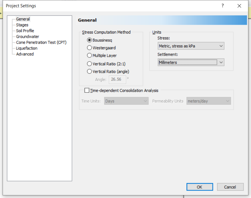
2. Ensure the General tab is selected.
3. Set the Stress units = Metric, stress as kPa and the Settlement units = Millimeters



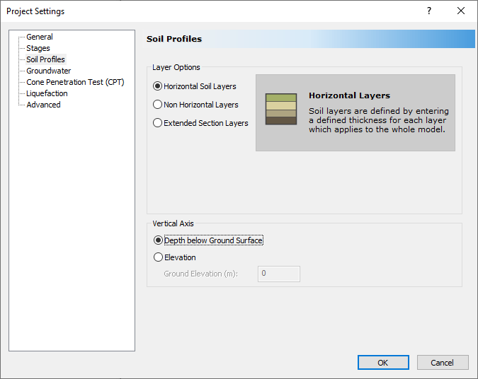
4. Now go to the Soil Profiles tab and select 'Depth below Ground Surface'.



5. You may be warned that the unit system has changed. If this is the case, select Yes to reset the unit-dependent values.
6. Click OK to close the Project Settings dialog.
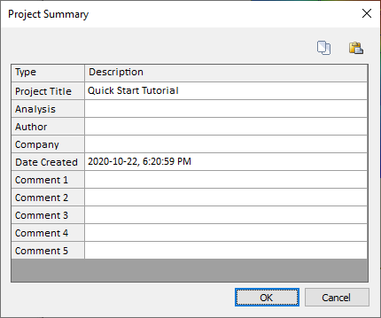
7. Select Home > Project Summary and enter “Quick Start Tutorial” as the project title.
8. Click OK to save your input and exit the dialog.

2.2 Adding a Load

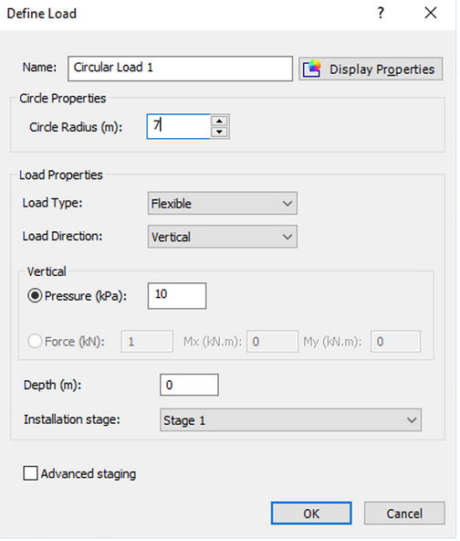
1. Select Loads > Circular Load
   
2. In the Define Load dialog, change the Circle Radius to 7 m.
   We will use the default of 10 kPa for the Vertical Pressure with a Load Type set as Flexible with a depth of 0 m (i.e. load is placed on the ground surface).
3. Click OK to close the dialog.



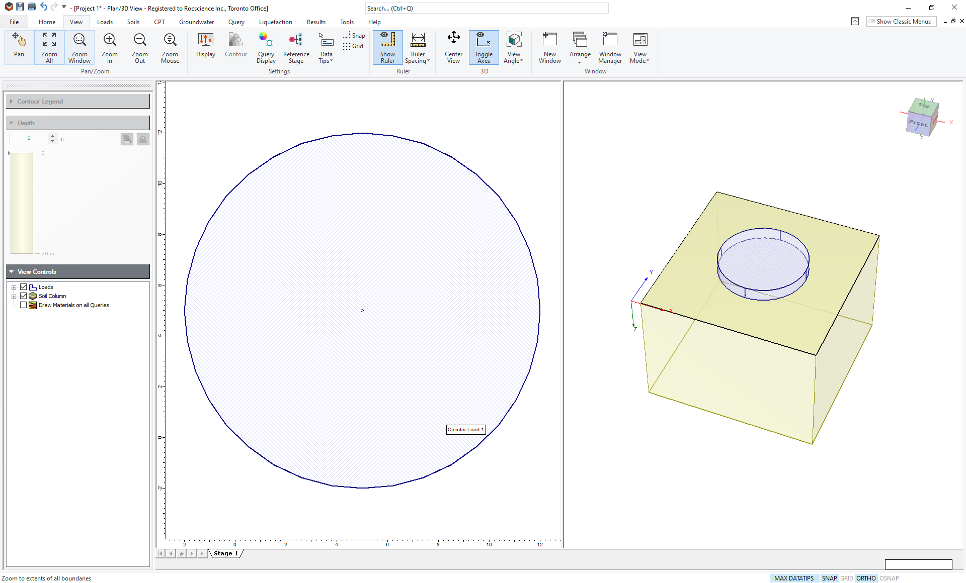
4. You will now see a circle that needs to be placed somewhere on the Plan View. You can click the mouse to place the circular load, or alternatively, you can enter the coordinates in the prompt line at the bottom right of the screen.
5. Enter 5,5 and hit Enter to place the center of the circular load at the coordinates (5,5) in the Plan View.
   
   You should now see the circular load in both the Plan View (left) and 3D View (right). You can zoom to the extent of boundaries by selecting the Zoom All toolbar button or pressing the F2 function key.
   
   
6. Select View > Zoom > Zoom All

Your model should now look like this:

2.3 Soil Properties

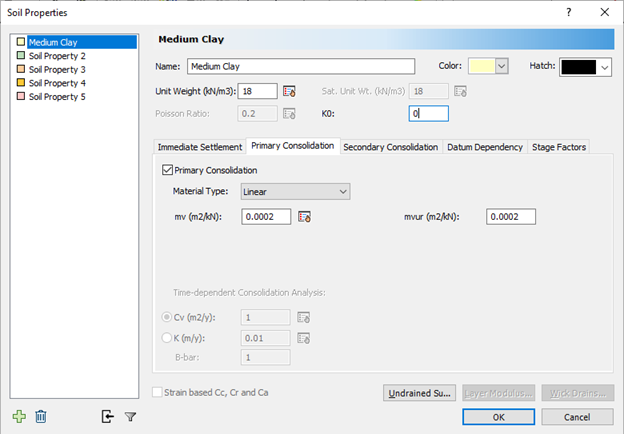
1. Select Soils > Define Soil Properties
2. Enter the following properties under the first tab of the dialog:
• Change the name of the soil to Medium Clay. Leave the default Unit Weight of 18 kN/m3
• You can use the checkboxes to enable or disable the input for Immediate Settlement, Primary Consolidation or Secondary Consolidation. If a checkbox is selected, then the corresponding settlement type will be computed for that material. By default, only the Primary Consolidation checkbox is selected.
• Select the Immediate Settlement checkbox. The parameters for immediate settlement determine the instantaneous settlement before consolidation starts. These are essentially undrained material properties. The parameter Es is the one-dimensional Young’s Modulus commonly used in settlement analyses. Leave the default values for Es and Esur (10000 kPa). (See the Settle3 help for detailed information about the input parameters.)
• The Primary Consolidation parameters determine the settlement that occurs as pore pressure dissipates and the soil compacts over time. In this tutorial, we are not looking at time-dependent consolidation so these parameters will only influence the long-term settlement after all excess pore pressure has dissipated (sometimes called ultimate settlement). Change the Material Type to Linear. For a linear material, we only need to specify mv, which is the one-dimensional compressibility. We will use the default parameter values (mv = 0.0002).



• For most of the material input parameters in the Soil Properties dialog, you will notice a Pick icon beside the input edit box. If you select this button, you will see a dialog with published test results for a variety of soil types. This allows you to obtain estimates of parameter values if you do not have your own analysis data. This is left as an optional exercise, after completing this tutorial
3. We are only defining a one-material model, so select OK to save the selections and close the dialog.

2.4 Soil Layers

To define the thickness and sequence of the soil layers:

1. Select Soils > Layers
2. Here you can add layers of different materials and change their thickness. We will specify only one layer of material but we will change the thickness to 25 m. The dialog should look like this:
   
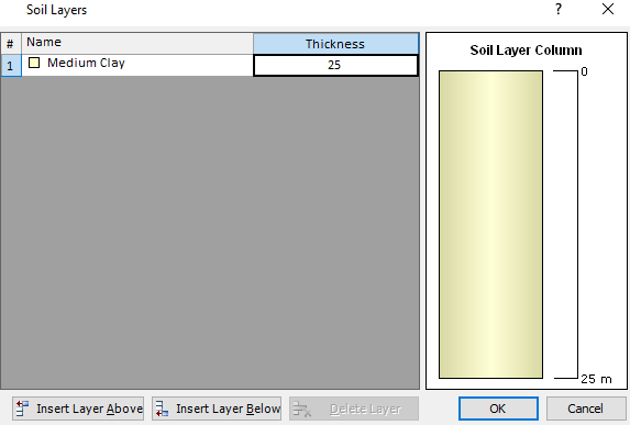
3. Click OK to close the dialog.

2.5 Field Point Grid

Stresses and strains are calculated on one-dimensional strings of points descending vertically from the ground surface. To compute results in 3D, an array of these 1D strings is required. The simplest approach is to automatically generate an array of strings by choosing Auto Field Point Grid from the Query menu.

1. Select Query > Auto Field Point Grid
   
   
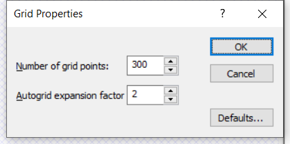
2. Click OK to accept the default values.
   

A grid will be generated while the stresses and strains are automatically computed throughout the 3-dimensional volume. By default, contours of Total Settlement will be shown. Your model should now look like this.

TIP: If you wish to view the location of the field points, go to View > Query Display Settings and under the Field Point Grid tab, choose a symbol other than None.

3.0 View Options

Before we proceed to examine the results, we will list some useful shortcuts for zooming, panning, rotating and maximizing the views:

Maximize Plan View or 3D View

• Within the Plan/3D View, you can quickly maximize the Plan View or the 3D View by double-clicking in the desired view

• To restore the split-screen presentation, double-click again in the maximized view

• You can also select the toolbar shortcut buttons – Expand Plan View, Expand 3D View, Split Plan/3D View - to maximize the Plan View, the 3D View, or restore the split-screen format.

Mouse Wheel Zoom

You can easily zoom in or out by rotating the mouse wheel forward or backward.

Mouse Wheel Pan

You can quickly pan the views by holding down the mouse wheel and dragging the mouse.

Rotate 3D View

You can rotate the 3D View by holding down the left mouse button and dragging the mouse in the 3D View.

Reset View

If you want to reset the default viewing angle of the model in the 3D View, right-click in the view and select Reset View from the popup menu. A variety of other viewing and display options are available through the right-click menu, the sidebar and other shortcuts, these can be explored after completing this tutorial.

4.0 Result Visualization

4.1 Total Settlement

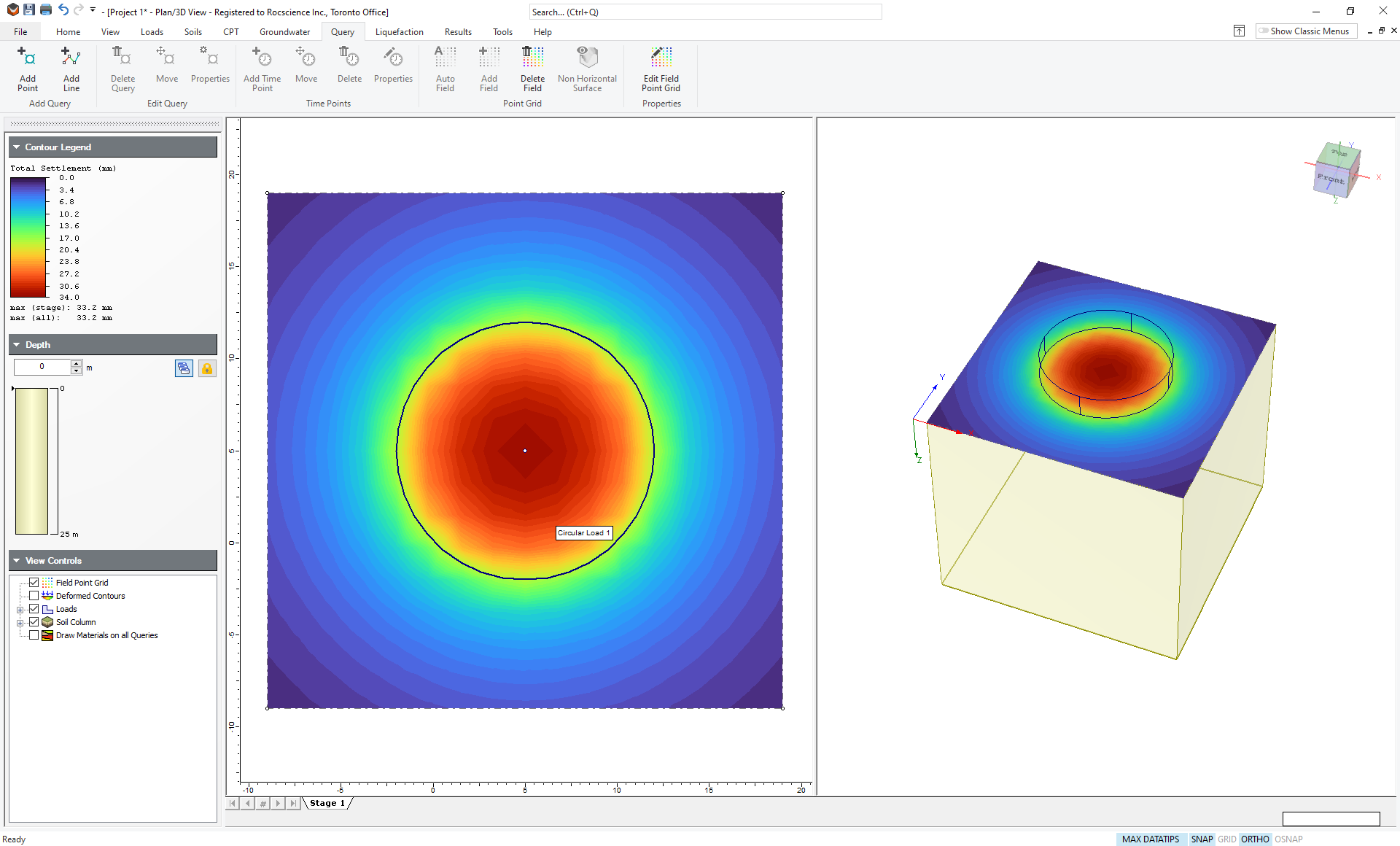
By default, contours in the Plan view and 3D View show the Total Settlement. Under the Contour Legend in the Sidebar, you can see that the maximum settlement is 33.2 mm. You can visualize this displacement in the 3D view by selecting the Deformed Contours checkbox in the View Controls in the Sidebar. If you rotate the 3D view (hold down the left mouse button and move the mouse), then you should see a screen like this:

TIP: The deformation of the surface is multiplied by a default scale factor. To change the scaling of this deformation, go to View > Query Display Settings > Field Point Grid > 3D View and change the Deformation Factor

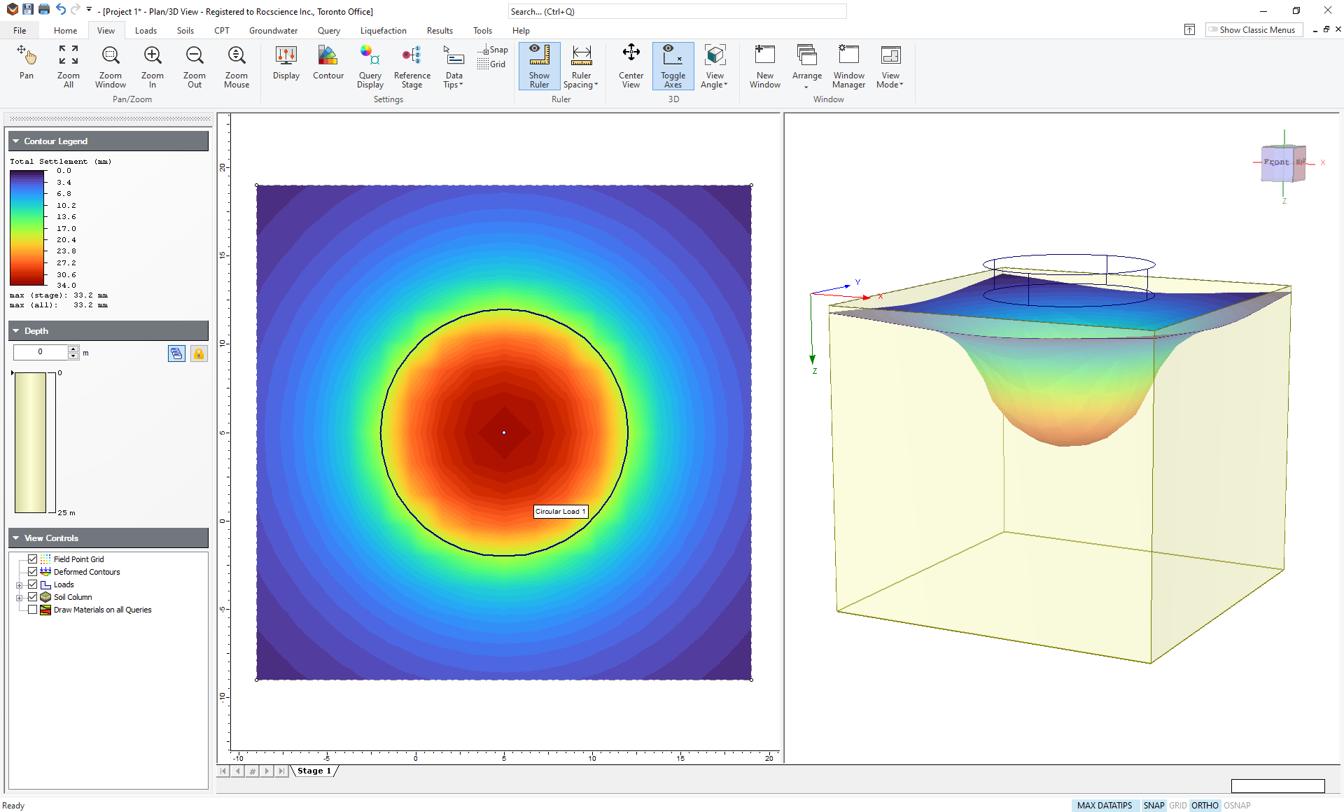
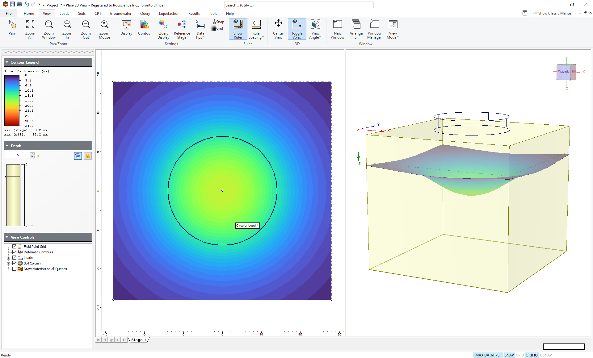
By default, the settlement at the ground surface (Depth = 0) is shown. You can examine the settlement at different depths by using the depth control in the Sidebar.

1. Change the depth to 5 m and the Settlement looks like this:

TIP: You can change the contour range, interval and color scheme by choosing Contour Options from the toolbar, View menu or right-click menu.

2. Turn off the deformed contour display, and reset the depth control to 0

4.2 Plotting Other Data Types

In the Results tab, you can change the data type being plotted. As well as Total Settlement you can use the drop down to select Immediate Settlement or Consolidation Settlement.

For this example, the Total Settlement is the sum of the Immediate Settlement and Consolidation (long-term or ultimate) Settlement. Therefore plotting either one of these will show less displacement than the Total Settlement. In this case, the maximum immediate settlement is 11.1 mm and the maximum consolidation settlement is 22.1 mm. As you can see from the contours, these values occur at the center of the flexible circular load.

You can also plot the Loading Stress or Total Stress. The Loading stress is simply the stress due to the load, whereas the Total Stress is the Loading Stress plus the stress due to gravity (i.e. self-weight of the soil)

4.3 Queries

To obtain results at specific locations, you can add Query Points or Query Lines. These allow you to graphically plot data versus depth or horizontal distance, at any location in the model.

4.3.1 Query Points

1. Select Query > Add Point

You will see the following Query Point dialog:

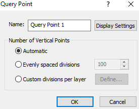
A Query Point is actually a vertical line that divides the soil layer(s) into sub-layers (divisions). Stress and displacement are calculated for each sub-layer. More divisions generally produce more accurate results. This dialog allows you to specify the number of divisions for each layer.

2. Leave the default choice of Automatic. This will generate subdivisions such that the discretization is denser near the ground surface where the high-stress gradients are likely to be.
3. Click OK and the cursor will become a cross-hair in the Plan View. You now need to specify the location of the Query Point on the surface. You can click the mouse at the desired location or you can manually enter coordinates in the prompt line at the bottom right of the screen. Enter the coordinates (5,5) to place the Query Point at the centre of the circular load.

If you are still viewing Total Settlement, your screen should now look like this:

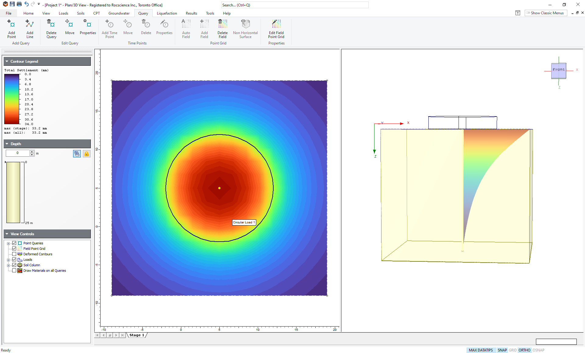
In the 3D View, you can see the Total Settlement plotted along the vertical line represented by the query point.

To graph the query data:

1. Select Results > Graph Query
2. Select the Query Point using the mouse and hit Enter. You will see the following dialog:
   
   
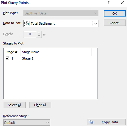
3. Choose Total Settlement if it is not already selected and hit OK. You should now see a graph that looks like this:
   

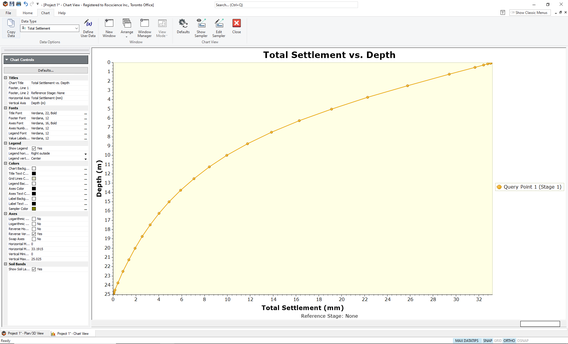
As expected the amount of settlement decreases with depth. At the bottom of the soil layer, the settlement is zero because the soil is assumed to be underlain by rigid bedrock. You can now easily plot other data by selecting from the list in the toolbar.

4.3.2 Query Lines

1. Toggle back to the model view by clicking the Plan 3D View tab at the bottom left of the screen.
2. Select Query > Add Line
3. You are first prompted for the number of horizontal divisions. Leave the default value of 20.
4. As with a Query Point, you are also prompted for the number of vertical divisions. This time select Evenly Spaced Divisions and change the number to 25.
   
   
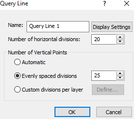
5. This will generate 20 vertical strings with 25 divisions in each string. Click OK and you will now be prompted for the start point of the line.
6. With the mouse, select the existing query point at the center of the circle. You will now be prompted to enter the second point.
7. Using the keyboard, enter the coordinates (5,-9). Hit Enter.
   

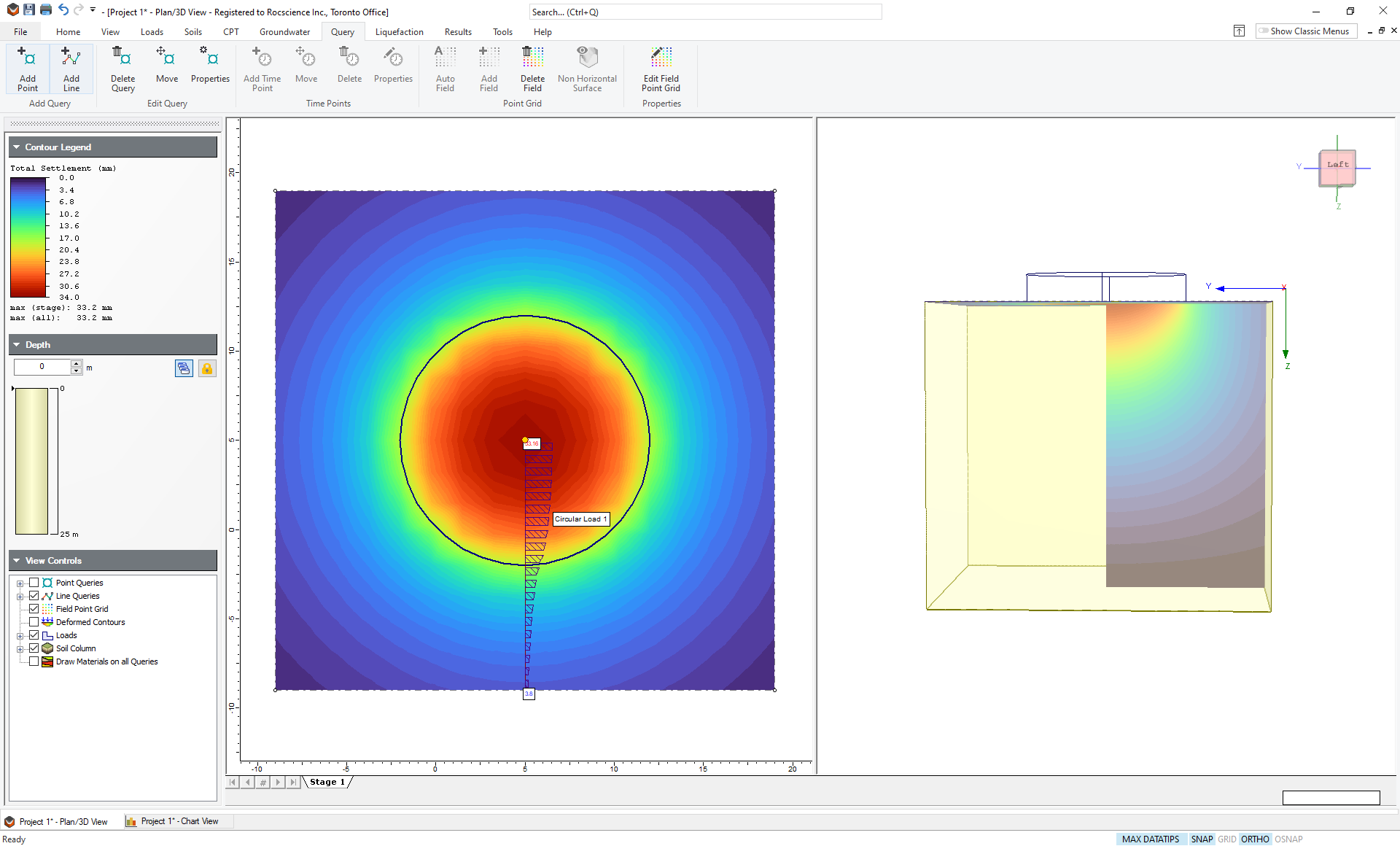
The Query line will appear on the Plan View with bars giving the Total Settlement along the line. The minimum and maximum values are shown numerically. The 3D View will show a vertical cross-section with contours of Total Settlement. To see this more clearly, turn off the Point Query display (clear the checkbox next to Point Queries in the Sidebar under View Controls), and rotate the model in the 3D View until the screen looks as follows:

8. You can plot the data by selecting Results > Graph Query and selecting the query line (or by right-clicking on the line and choosing Graph Query).
9. Choose the data you wish to plot (Total Settlement) and click OK.
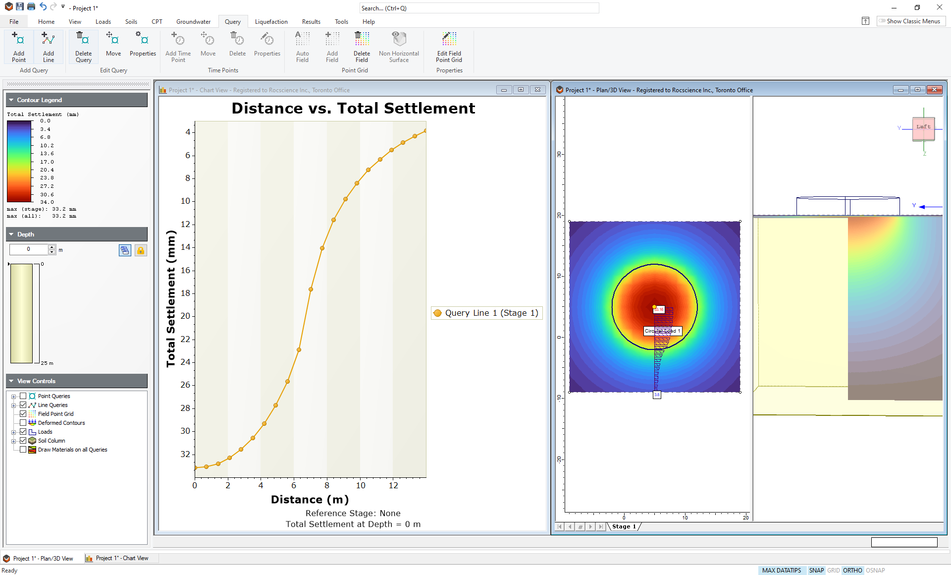
10. You will see a graph showing the Total Settlement versus horizontal distance along the line, at the current depth. In the Sidebar under Axes, change the horizontal and vertical values to the following:

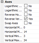
Your graph should now look like this:

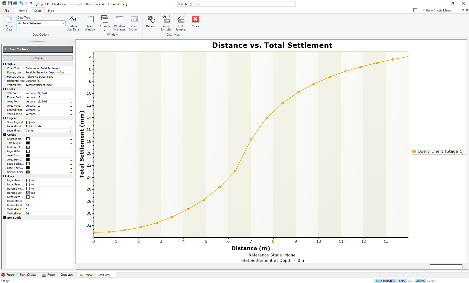
This is the Total Settlement along a line at the ground surface.

You can change the depth of the line by using the depth control in the Sidebar of the Plan View. You can also change the data being plotted using the drop-list in the toolbar. Close any extra windows so that only the Plan View window and query line chart windows are open. Tile the windows so that they look like the window below.

11. Select Chart > Arrange > Tile Windows Vertically



12. Click on the Plan View window, and the depth control sidebar will appear.
13. Change the depth to 5 m. Both the Plan View and Chart View results will change to those at 5m.
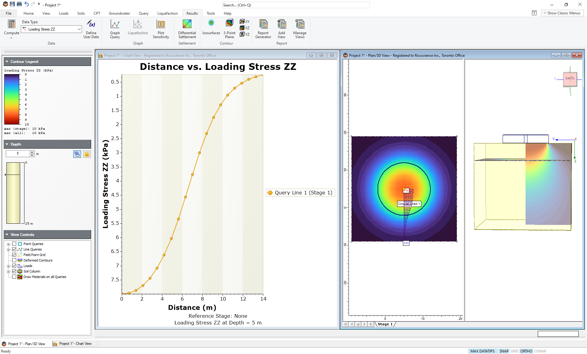
14. Click on the Chart View and change the dropdown results type to Loading Stress ZZ.
15. Click on the Plan View window, go the Results tab and do the same.

You are now looking at the contour and query line results for Loading Stress ZZ at a depth of 5m. The window should look like the figure below

TIP: You can export this data to a Microsoft Excel spreadsheet by simply right-clicking on the graph and choosing Plot in Excel. If you prefer another spreadsheet program, then choose Copy Data and you will be able to paste it into any Windows program

5.0 Report Generator

The Report generator presents a formatted summary of input data and analysis results.

To open the Report Generator:

1. Select Results > Report Generator

The toolbar contains the Report Generator Controls, which allow you to select what information is displayed, and customize the appearance.

The data can be exported in a variety of ways: it may be manually copied, viewed in a browser, printed, or the information may be saved as a .pdf file. Prior to printing the file, results may be formatted to your specifications.

Click on the Close window icon in the Report Generator toolbar to close the viewer and return to the model view.

6.0 Drawing Tools

As a final exercise, we will mention the Drawing Tools which allow you to add a variety of drawing objects to the Plan View. For example, you can add a table of soil properties. To begin, switch back to the Plan/3D View.

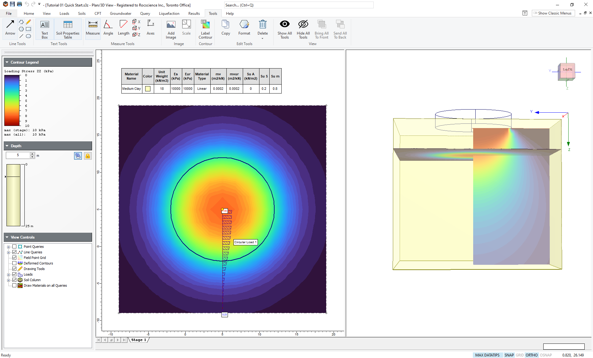
1. Select Tools > Soil Properties Table

2. Click the mouse in the Plan View to add the table, as shown in the figure below.

3. After adding the table, it can be edited, moved or formatted (e.g. double-click on the table to display the Format Tool dialog). See the help for more information.

This concludes the Quick Start Tutorial; you may now exit the Settle3 program.