Analysis of Triaxial Field Data

1.0 Introduction

This tutorial will fit the Generalized Hoek-Brown criterion to triaxial strength data for a rock mass.

Finished Product:

The finished product of this tutorial can be found in the Tutorial 4.rsdata data file. All tutorial files installed with RSData can be accessed by selecting File > Recent Folders > Tutorials Folder from the RSData main menu.

2.0 Creating the model

1. Open the RSData program.
2. Select the Rock Template and click OK.

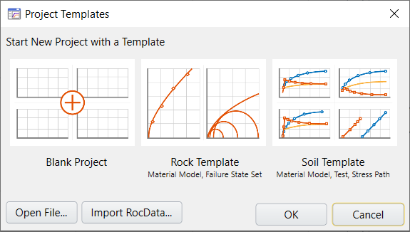
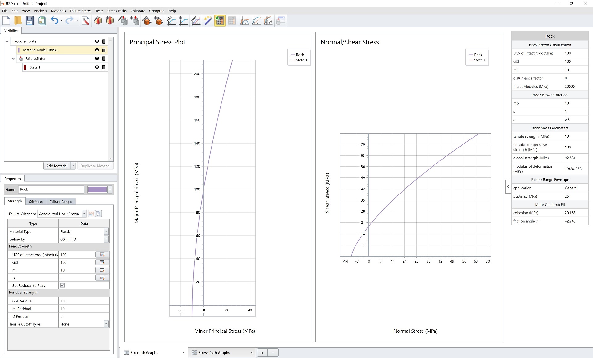
By default, strength graphs are presented and a rock template is given for Rock Project Template. Within the rock template, a rock material model and an empty failure state are included. The rock material is also depicted on the strength graphs.

3.0 Failure State

We will input the field data points into the Failure state.

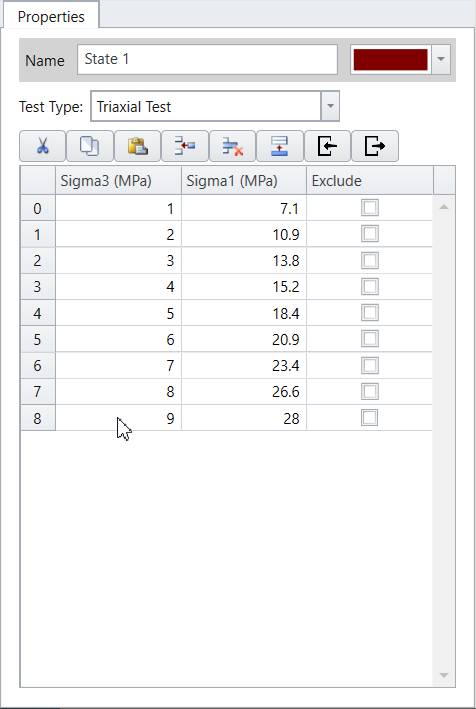
1. In the Visibility Tree, go to the Failure States and select State 1.
2. In the properties panel below, select Test Type = Triaxial Test
3. Enter the following triaxial data points in the data grid:

	Sigma3 (MPa)	Sigma1 (MPa)
0	1	7.1
1	2	10.9
2	3	13.8
3	4	15.2
4	5	18.4
5	6	20.9
6	7	23.4
7	8	26.6
8	9	28

Triaxial data points are drawn as points on the Principal Stress Plot representing the failures and as Mohr circles on the Normal vs. Shear Stress graphs as follows:

4.0 Calibration– Generalized Hoek-Brown

The next step is to curve fit/calibrate the field dataset and find the best fit failure envelopes with Generalized Hoek-Brown method.

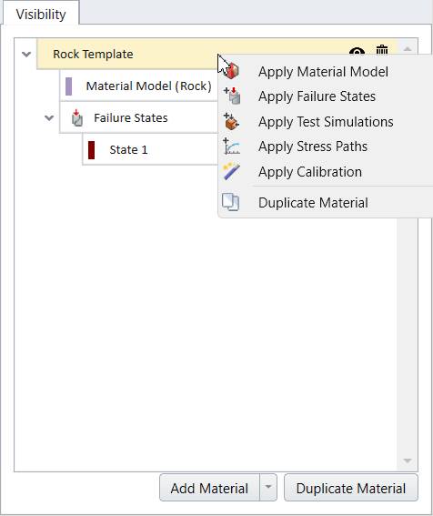
1. Under the visibility tree, right click on Rock Template, and select Apply Calibration.



2. A Calibration set is added to Rock Template. Select the added Calibration set and in the properties section below, enter the following:
• Calibration strength type = Generalized Hoek-Brown.
• Failure data type = Field Data

Note: In this tutorial, the given data is field data.

A section of sigci (MPa) and D values will need to be filled in for field data calibration.

3. Input the values given as:

• Sigci (Mpa) = 50
• D = 0.5
• Algorithm = Modified Cuckoo
• Error Summation = Vertical
• Error Type = Absolute

The calibration properties section should look as follows:

5.0 Results

By default the Auto Compute is selected and the result will be updated. The user has control to toggle the Auto Compute on and off. If Auto Compute is toggled off, be sure to select Compute to compute the calibration.

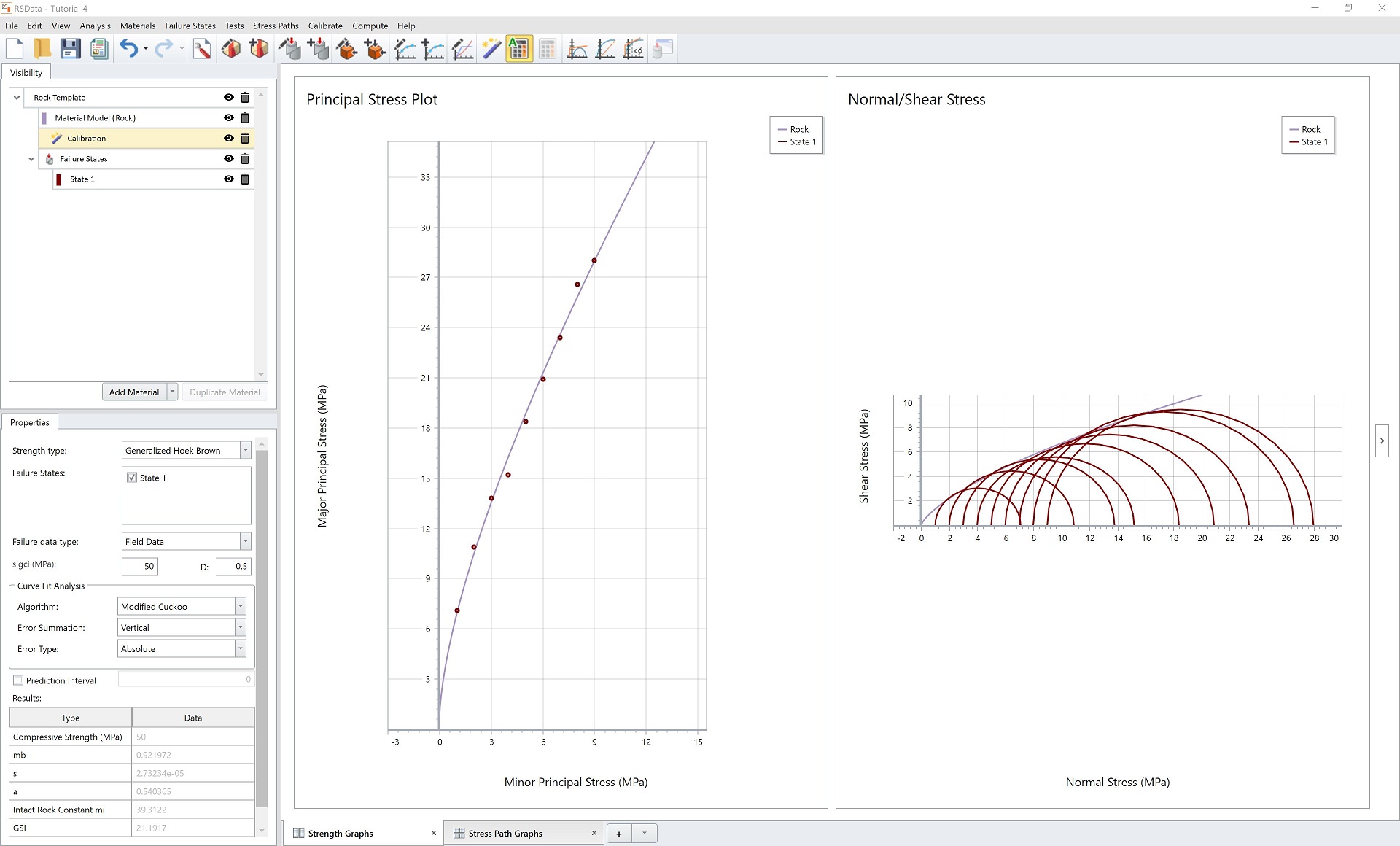
The numerical calibration results are summarized in the table under calibration properties section (as shown above). The results are also shown in the collapsible chart on right side panel.

The calculated parameters are:

• Compressive Strength = 50 MPa
• mb = 0.92
• s = 2.73e-05
• a = 0.540
• Intact Rock Constant mi = 39.31
• GSI = 21.19
• Residuals = 2.46

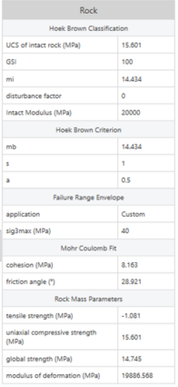
The calibration results will also be updated to the material model. We can check by viewing the Material Mode (Rock) properties dialog as below. The Strength parameters and Failure Range parameters are recalculated.

Note: You can also select the Material Model (Rock) in the visibility tree to view the results in the properties pane.

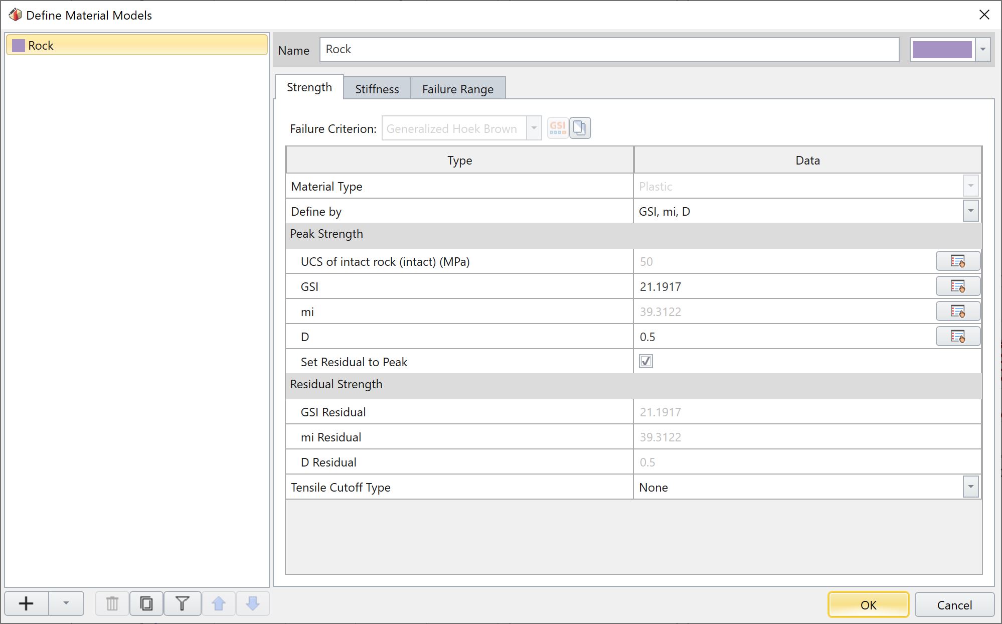
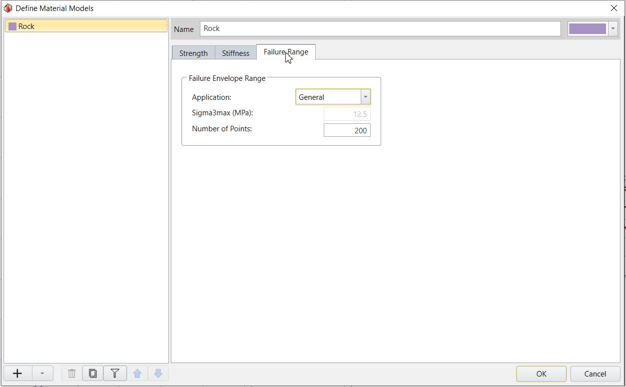
Click OK to close the dialog.

GRAPHICAL CALIBRATION RESULTS

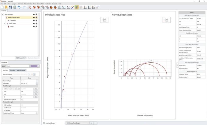
Failure envelopes are also updated on the Principal Stress Plot and Normal vs. Shear Stress Plot as displayed below.

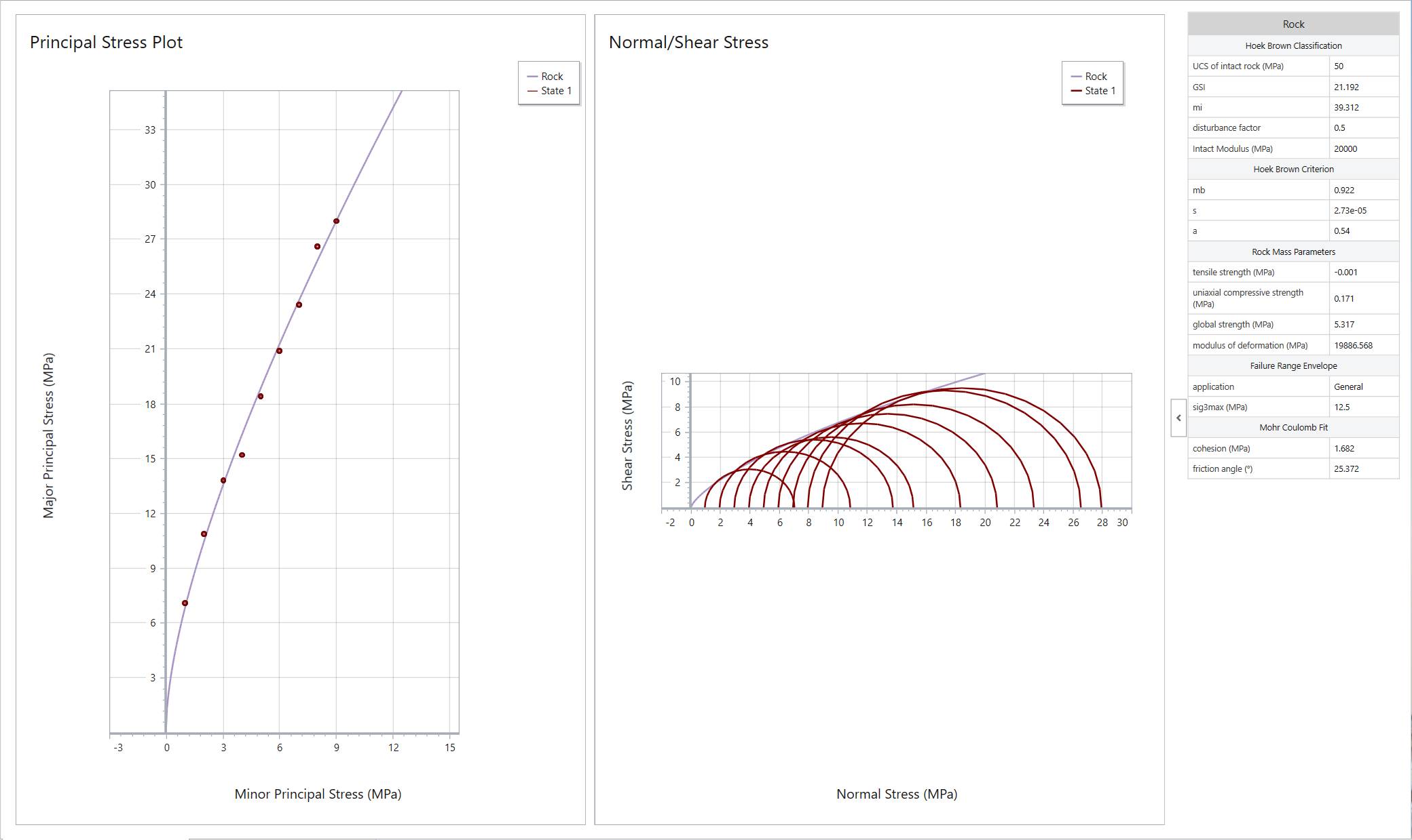
For both plots, the calibrated failure envelopes are depicted in a purple line. In the Principal Stress Plot, it can be observed that the line is fitting the field dataset well.

Users can double click on each graph for a closer look.

Here concludes the RSData Tutorial – Generalized Hoek-Brown Analysis of Triaxial Field Data, where triaxial field data for a rock mass was calibrated in RSData with the Generalized Hoek-Brown method.