Application of Joint Networks (with XFEM)

1.0 Introduction

This tutorial will demonstrate how to specify joint networks or discrete fracture networks (DFN) in RS2 using XFEM. It will also demonstrate techniques for analyzing the effects of joints on model results. The model involves the stability analysis of slope contained of a parallel joint network.

2.0 Constructing the Model

1. Select File > Recent Folders > Tutorials Folder > Jointed Rock
2. Select Jointed Slope with XFEM (Initial)

2.1 PROJECT SETTINGS

1. Select: Analysis > Project Settings to open the Project Settings dialog.
2. Select Solver Options and ensure that the Use XFEM checkbox is checked.
   
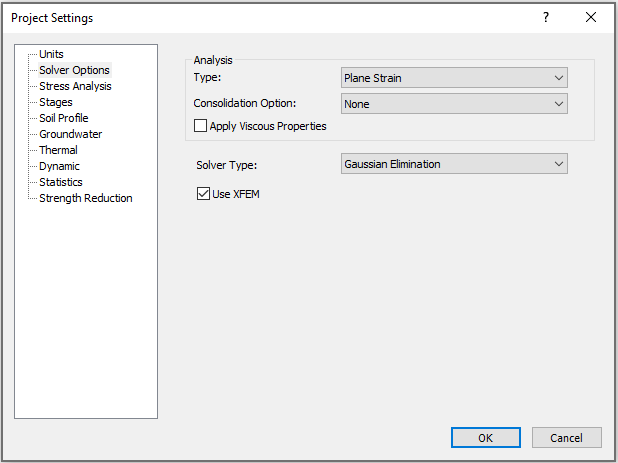
3. Click OK to close the dialog.

2.2 JOINT NETWORK PROPERTIES

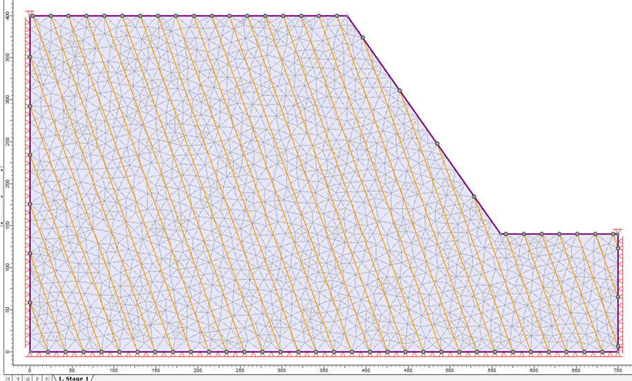
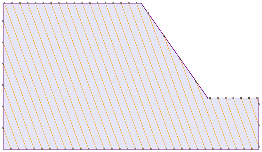
A joint network has been added to the model as orange hatched area using Boundaries > Joint Networks > Add Joint Network. For detail steps on adding a joint network, see the RS2 User Guide - Add Joint Network topic.

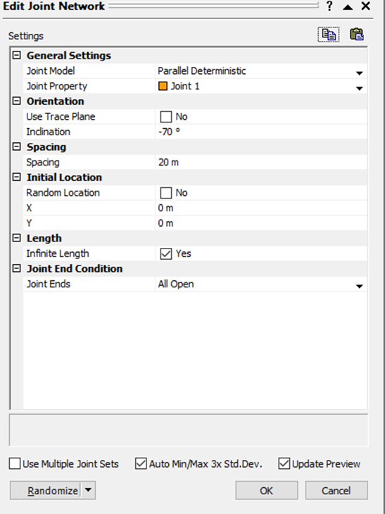
1. Right click on the joint network, select Edit Joint Network. In the Edit Joint Network dialog, the properties have been inputted as follows:



2. Do not change anything and click Cancel to exit the dialog.

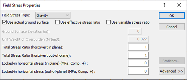
2.3 FIELD STRESS

1. Select Loading > Field Stress
2. For Field Stress Type, select Gravity and ensure only “Use actual ground surface” is checked.
1. Set Total Stress Ratio (horiz/vert in plane) = 1.0
2. Set Total Stress Ratio (horiz/vert out-of-plane) = 1.0
3. Select Ok to save and close the dialog.

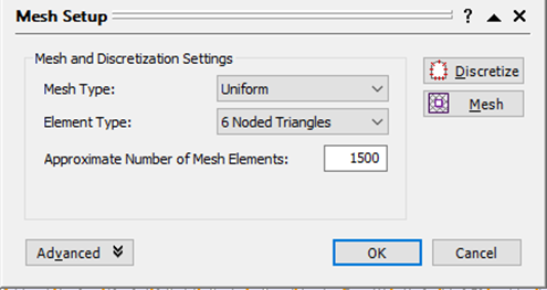
2.4 MESH

1. Select Mesh > Mesh Setup
2. In the Mesh Setup dialog:
1. Change the Mesh Type to Uniform and Element Type to 6 Noded Triangles in the drop-down menu
2. Enter the Approximate Number of Mesh Elements as 1500.
3. Select Discretize. If a Joint Networks Warning dialog appears, click “Clean geometry.” In the Geometry Cleanup dialog, accept the default values and click OK. Select Yes to the discretization and mesh prompt which follows.
3. Select Mesh > Mesh.

2.5 BOUNDARY CONDITIONS

By default, all nodes on the external boundary are pinned (fixed, zero displacement).

The slope (ground) surface must be free to move in any direction.

1. Select Displacements > Free
2. In the Set Restraints/Displacements dialog:
1. Ensure Selection mode = Boundary Segments.
2. Use the mouse to select all the top line segments defining the ground surface. Select Apply or right-click and select Apply in the drop-down menu.
3. Keep the Set Restraints/Displacements dialog open.
3. On the Set Restraints/Displacements dialog select the Restrain X,Y symbol (or if the dialog was closed select Displacements > Restrain X,Y).
4. Ensure Selection mode = Boundary Segments.
5. Select the line segments making up both the left and right vertical sides of the model. Select Apply and Close.

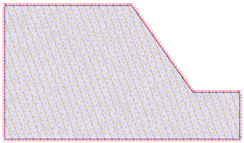
The resulting model should look like the following:

3.0 Compute

1. Select File > Save As
2. Select Analysis > Compute

4.0 Results and Discussion

1. Select Analysis > Interpret

4.1 CONTOURS OF MAJOR PRINCIPAL STRESS – SIGMA 1

The maximum compressive stress (sigma 1) would be displayed.

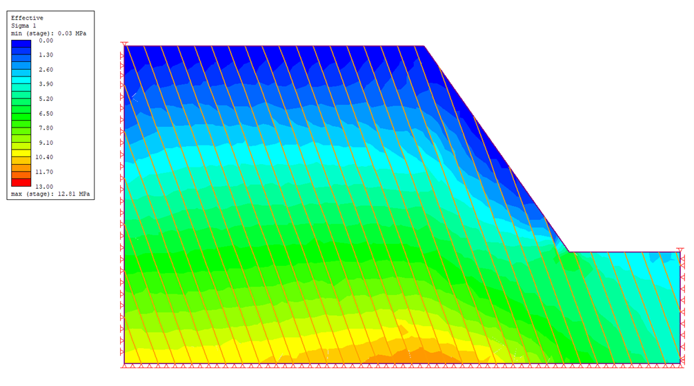
The effects of the joints on the Sigma 1 contours are visible; the contours are jagged and not as smooth as those for models without joints.

4.2. YIELDED JOINT

By clicking on yield joint icon, the yield joints in domain would turn to red and would display on active contour.

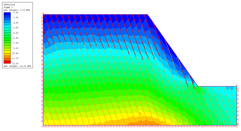
As it can be seen, more joints on the top part of the slop are yielded since they experience more deformation than joints at the bottom of the slop.

4.3. TOTAL DISPLACEMENT

1. Select Total Displacement from the drop-down menu in the toolbar.

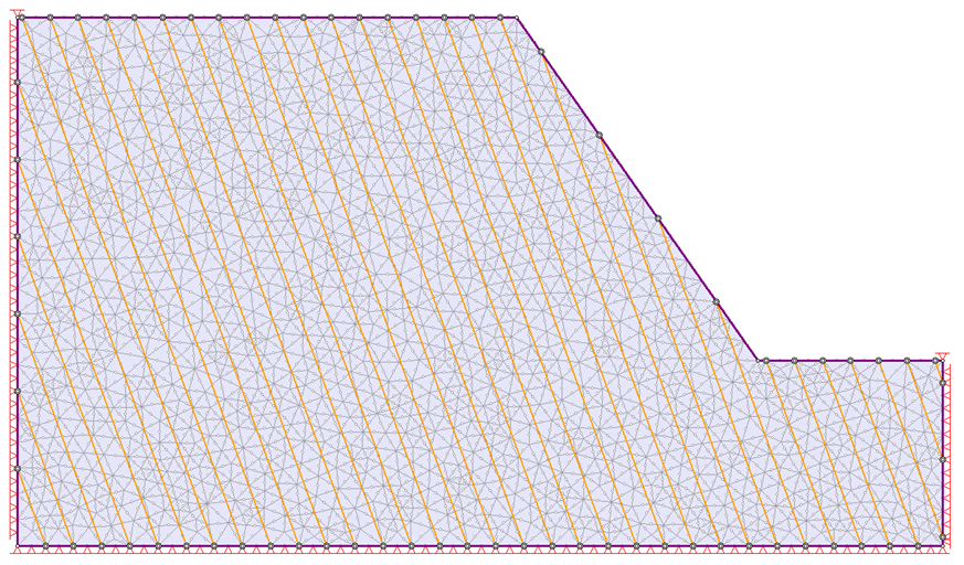
The contour would show the maximum deformation on the slop and zero deformation on the boundaries as they are set to be zero by assigning the boundary condition. As it can be seen, regarding to the presence of joints, the deformation is discontinuous in the domain. To compare the results of XFEM with regular explicit joints in FEM, we repeated the similar simulation, but this time the checkbox of “use XFEM” in project setting has turned off.

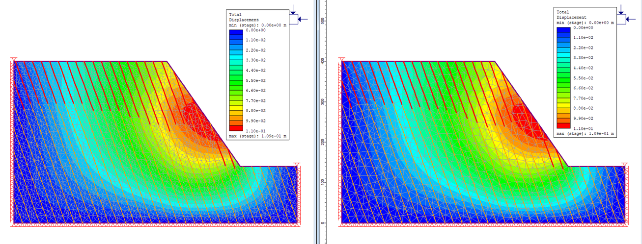
(Left) regular explicit joint and (right) XFEM

The mesh used for each analysis is displayed on the above figure. In the explicit joint, the mesh is aligned with the joint, however, in XFEM, joints are crossing the elements and it is not required to be aligned with joints. As it can be seen, the results are similar for both methods.