Drawdown Analysis for Tunnel Excavation
1.0 Introduction
In this tutorial, RS2 is used to simulate tunnel excavation in a saturated soil. The tunnel is assumed to have a permeable liner so there is a drawdown in the water table as water drains into the tunnel. The model is based on a study presented by Shin et al. (2002).
2.0 Constructing the Model
Select: File > Recent Folders > Tutorial Folder
Select: Drawdown Analysis for Tunnel (Initial) file
The geometry, material properties, and project settings have already been specified for this model.
2.1 Hydraulic Material Properties
![]()
 Select: Properties > Define Hydraulic
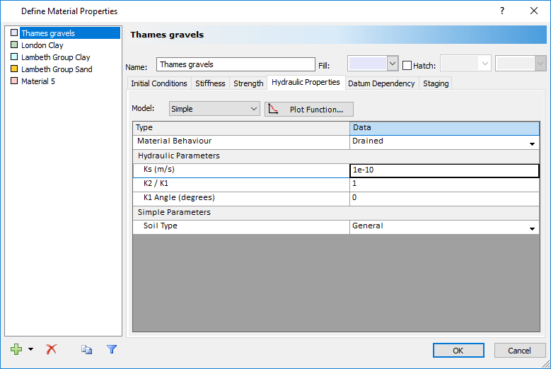
Select Thames Gravel. Here, it is possible to select the model that dictates the permeability transition from saturated to unsaturated soil. Leave the model as the default (Simple). Permeability can also be changed here. Set the value to 1e-10 m/s.
Click on the tab for London clay. The base permeability for the London clay is 1e-10 m/s. The permeability decreases by two orders of magnitude between 50kPa and 100 kPa of suction. This behaviour can be simulated with a user-defined permeability model. Set the Model to User Defined. Select "Define..." and fill in the parameters shown below:
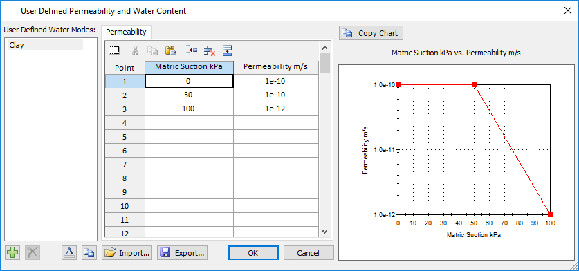
Click OK to return to the Define Hydraulic Properties dialog.
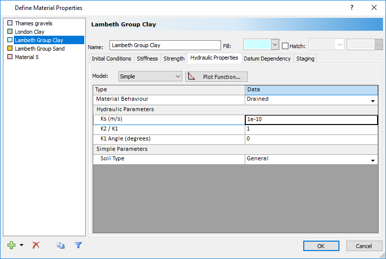
Click on the tab for Lambeth Group clay. Leave the model as Simple and set the permeability to 1e-10 m/s.
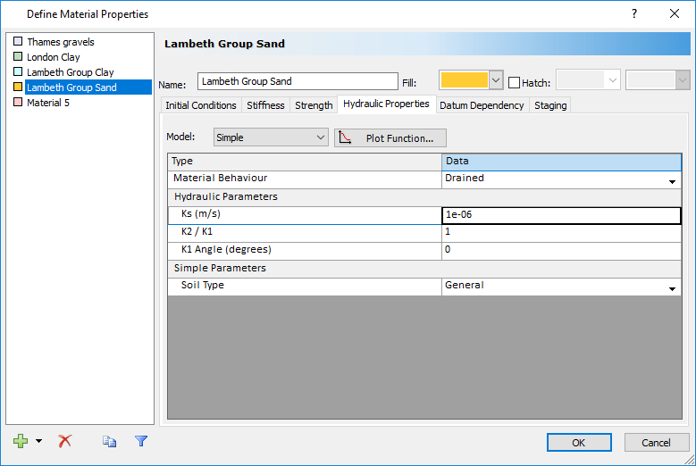
Click on the tab for Lambeth Group sand. Set the permeability to 1e-6 m/s as shown.
Click OK to close the dialog.
2.2 Excavation and Support
![]()
In general, a tunnel must be excavated before structural support is added. Therefore, some deformation will occur before the support is installed. The amount of deformation depends on the distance of the tunnel face from the location of support installation. The tunnel face provides some support, so if the liner is installed close to the tunnel face, then not much deformation will have occurred. In essence, this is a three-dimensional problem that we are trying to simulate in two dimensions.
For this problem, let’s assume that we are installing the liner 2 m behind the face. To simulate the supporting effect of the nearby tunnel face, we will apply a load to the perimeter of the tunnel equal to some proportion of the in-situ stress. The amount of load required to correctly simulate the 3D effect of the tunnel face can be determined by following procedures outlined in the 3D Tunnel Lining tutorial.
In the third stage, we will install the liner and remove the load. Removing the load will simulate the advance of the tunnel face away from our two-dimensional slice.
 Select: Loading > Induced Loads > Add Induced Stress Load
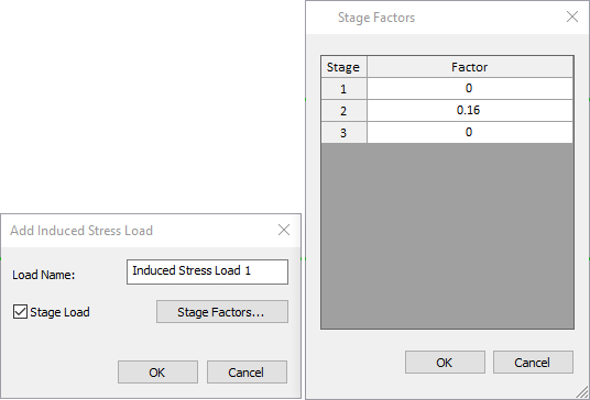
Click the check box for Stage Load. Click on the Stage Factors button. Through the type of analysis described in the Tunnel Lining Design tutorial, we can determine that a load of 0.16 times the in-situ stress will simulate the effective support of the tunnel face 2 m away. Therefore for Stage 2, set the Stage Factor to 0.16. For Stage 3, we assume that the tunnel face is far away so set the Stage Factor to 0.
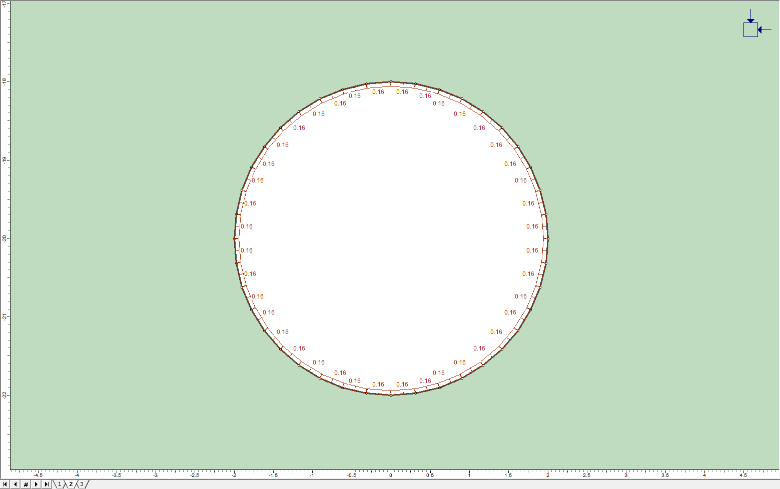
Click OK to close the dialog. Click OK to close the ‘Add Distributed Load’ dialog. You will now be prompted to select a boundary on which to apply the load. Click on the tunnel boundary and drag the mouse around the perimeter of the excavation to draw the load. If necessary, enter "f" in the prompt line to flip the orientation of the load. Press Enter to select the tunnel boundary. Press F6 to zoom in to the excavation. The model for Stage 2 should now look like this:
FIELD STRESS
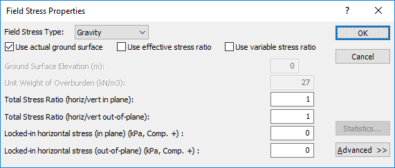
Because the top of the model represents the true ground surface, we want to use a gravity field stress.
 Select: Loading > Field Stress
For Field Stress Type select Gravity and click the check box for “Use actual ground surface”. Leave all other values as default.
2.3 Mesh
![]()
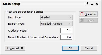
 Select: Mesh > Mesh Setup
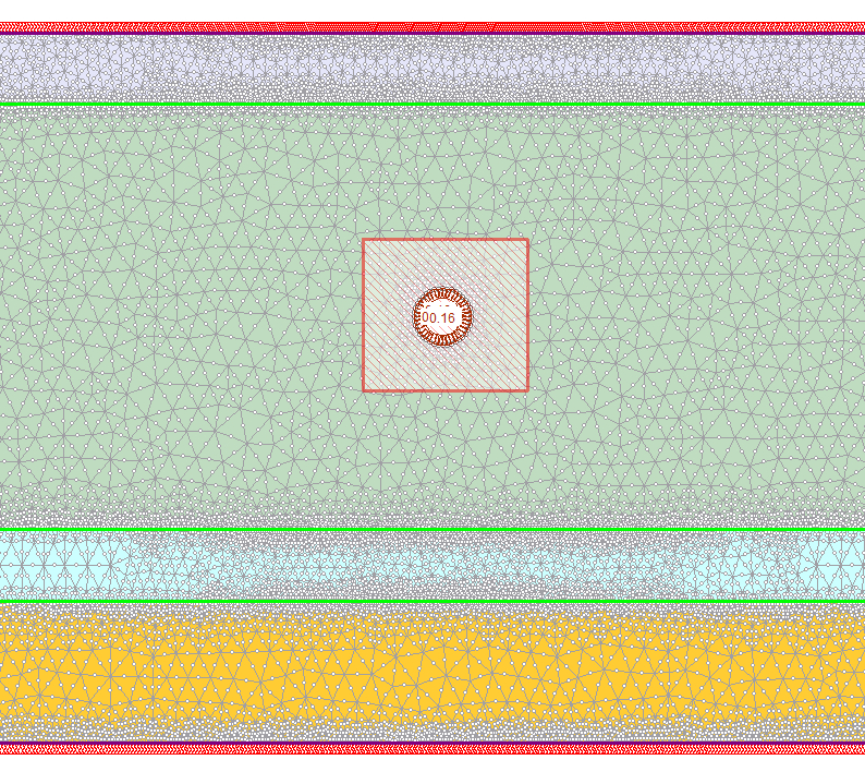
Change the Mesh Type to Graded. Leave the default element type (6 Noded Triangles) but set the number of elements to 110 with a Gradation Factor of 0.1. Click the Discretize button followed by the Mesh button.
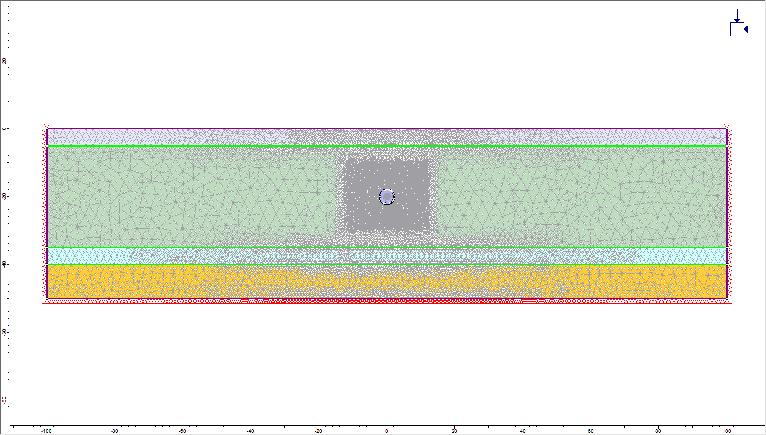
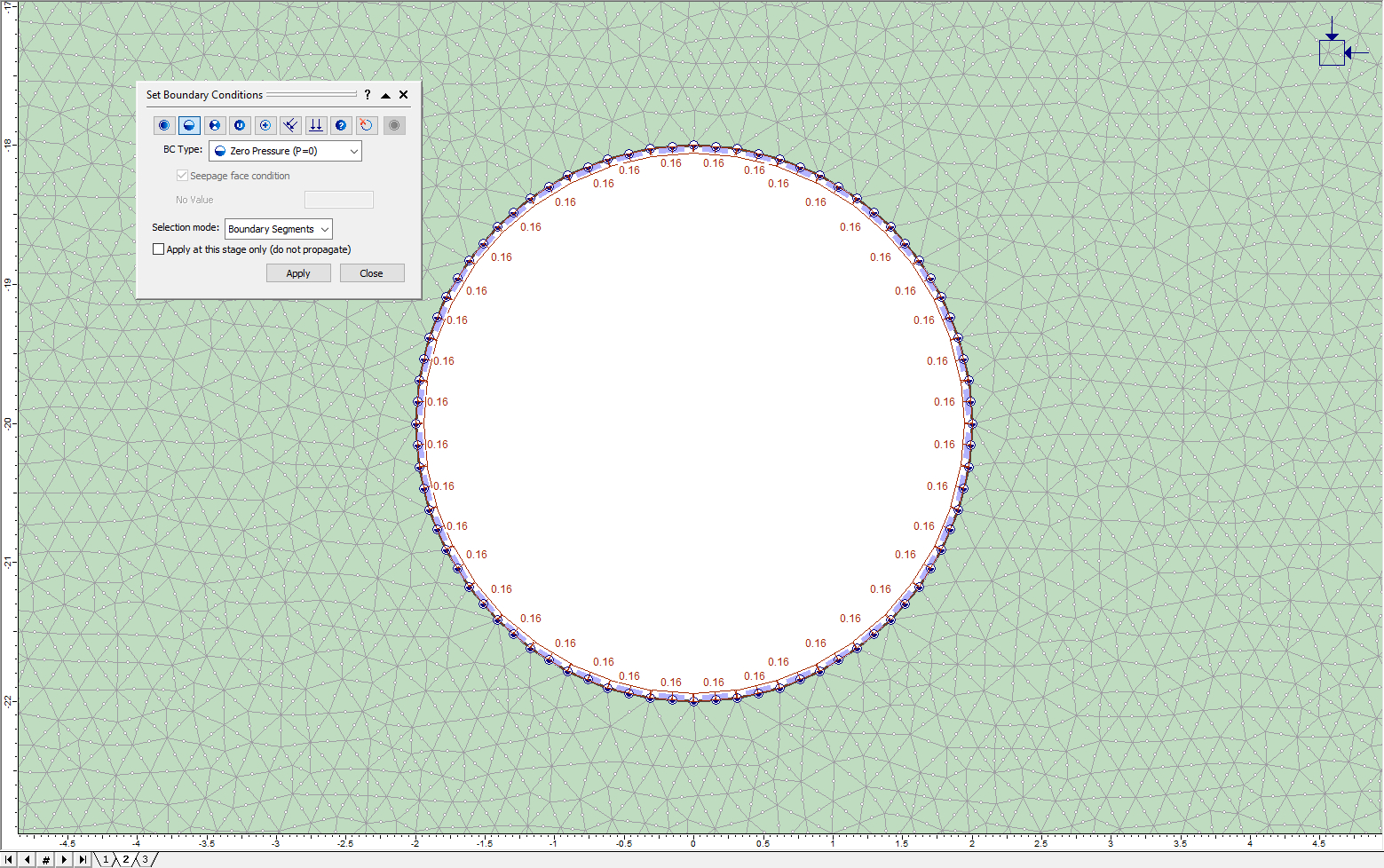
Because the area of interest is relatively small compared to the size of the model, a finer mesh should be used around the excavation. In the mesh properties dialog, select the advanced box. Click on the green plus sign to add an Advanced Mesh Region. Select a square around the excavation using the cursor:
Fill in the following properties in the Mesh Setup dialog:
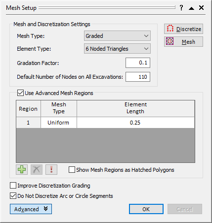
After adding the Advanced Mesh Region, the model should look like below:
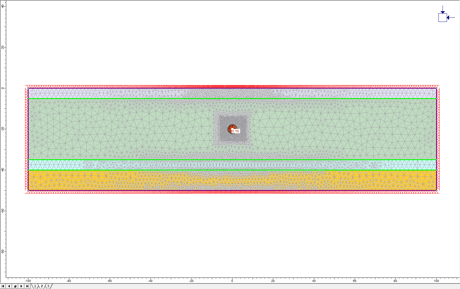
Close the Mesh Setup dialog by selecting the OK button.
2.4 Add Composite Liner
![]()
Click on the Stage 3 tab. To add the composite liner:
![]() Select: Support > Add Liner
Select: Support > Add Liner
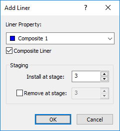
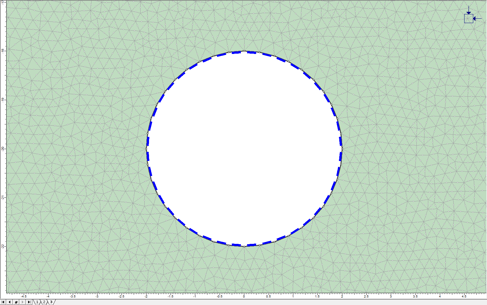
Tick the box for Composite Liner and ensure that the liner will install at stage 3. The default liner and joint properties will be used, so there is no need to define them prior to adding the composite liner.
Draw a selection box to install the liner on the excavation boundary. The model (Stage 3) should look as follows:
2.5 Groundwater Boundary Conditions
![]()
The water table for this site is 2.5m below the ground surface. This can be set up using groundwater boundary conditions. Ensure Stage 1 is selected and press F2 to zoom out to view the entire model.
 Select: Groundwater > Set Boundary Conditions
For the BC Type, choose Total Head. Set the Total Head Value to -2.5 m.
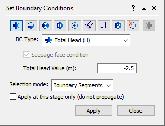
Select all sections of the left and right vertical boundaries. Click Apply. The model will appear as shown: 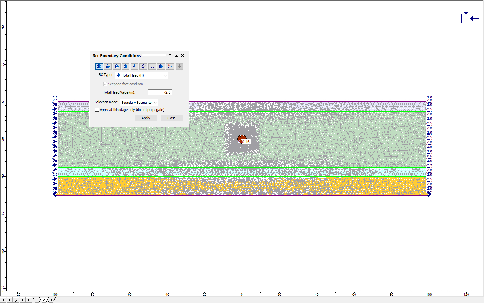
To simulate the effect of a permeable liner, the pressure at the surface of the tunnel will be set to 0. Select the Stage 2 tab. From the Set Boundary Conditions dialog, select BC Type = Zero Pressure.
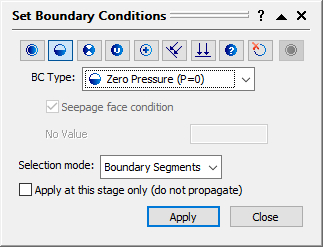
Use the cursor to draw a selection window around the tunnel. Click Apply, then close the dialog. The model should look like this:
Click on the tab for Stage 3 to ensure that the zero pressure boundary condition also exists in this stage.
2.6 Boundary Conditions
![]()
The model now shows the default boundary conditions (all external boundaries fixed in the x and y directions). To free the ground surface of this model:
 Select: Displacements > Free
Click on the ground surface and press Enter. The fixed boundary conditions have now disappeared from the top boundary.
The top left and top right nodes of the soil layer have now been freed. To re-fix them, select Restrain X, Y from the Displacements menu and click on the left and right edges of the soil layer (make sure that the selection method is set to "boundary nodes" in the right-click menu). Hit Enter to finish. The model should now look like this:
The model definition is now complete. Save the model using the Save As option in the File menu.
3.0 Compute
![]() Select: Analysis > Compute
Select: Analysis > Compute
4.0 Results and Discussion
![]() Select: Analysis > Interpret
Select: Analysis > Interpret
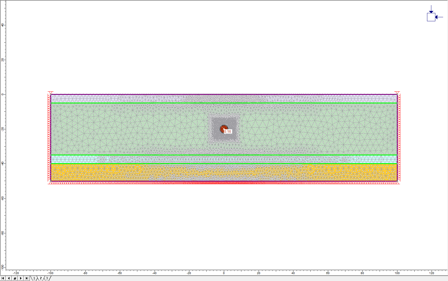
The Pressure Head results for Stage 1 are displayed below (select Seepage > Pressure Head from the drop-down menu in the toolbar)
As expected, the water table (pink line) is at 2.5 m below the surface and the pressure increases monotonically with depth. Click on the tab for Stage 2.
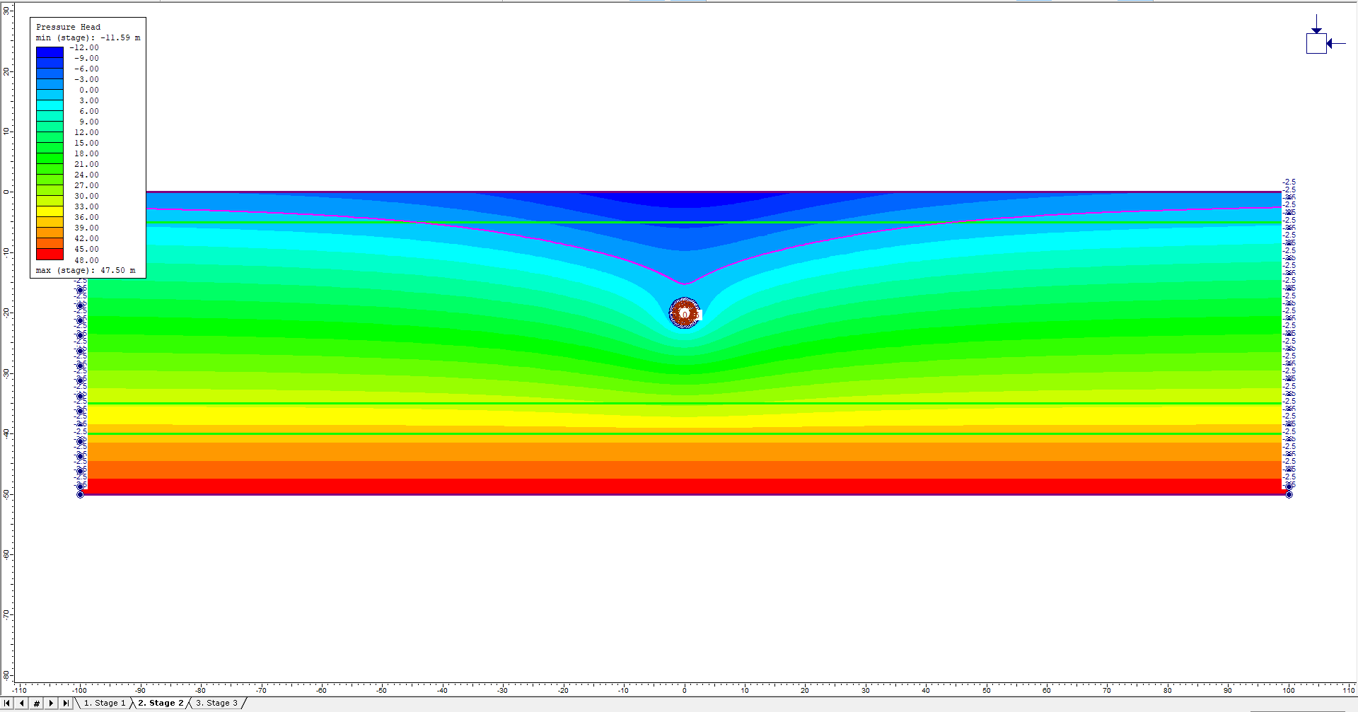
Here you can see the obvious drawdown of the water table due to the drained boundary around the tunnel.
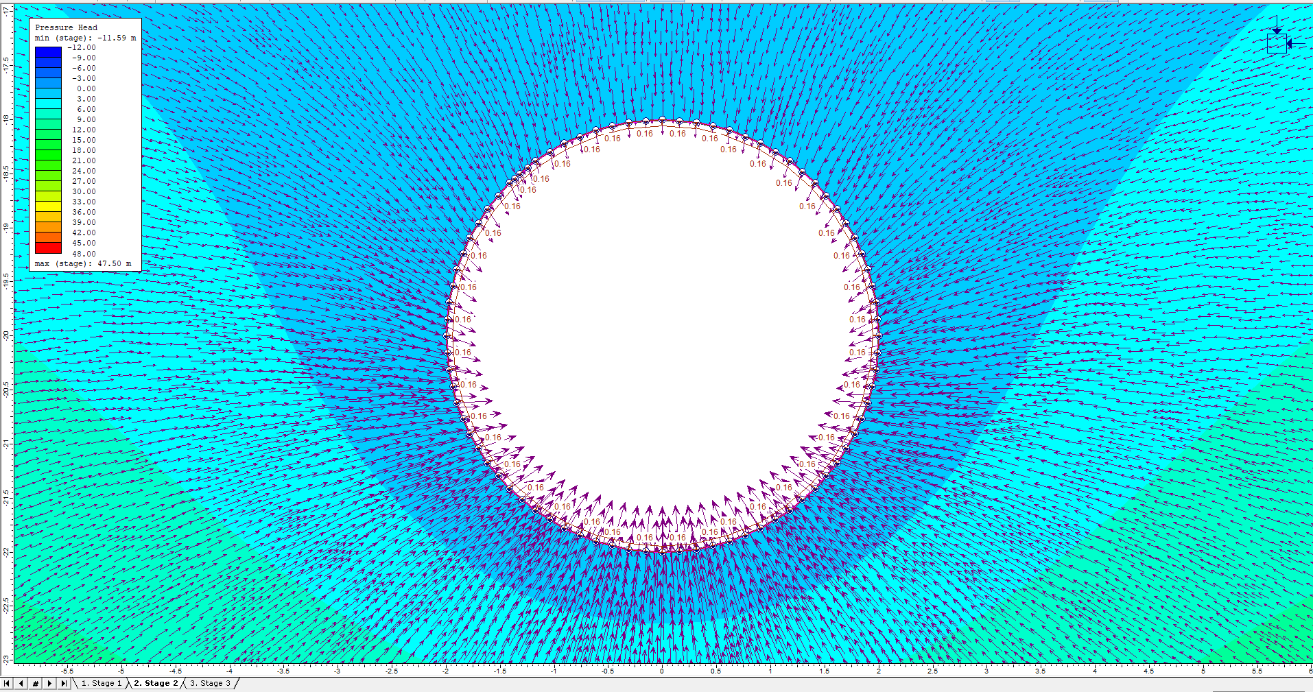
Show the flow vectors by clicking on the Show Flow Vectors button in the toolbar. Zoom in on the tunnel (F6) and you can see how the fluid is flowing into the tunnel.
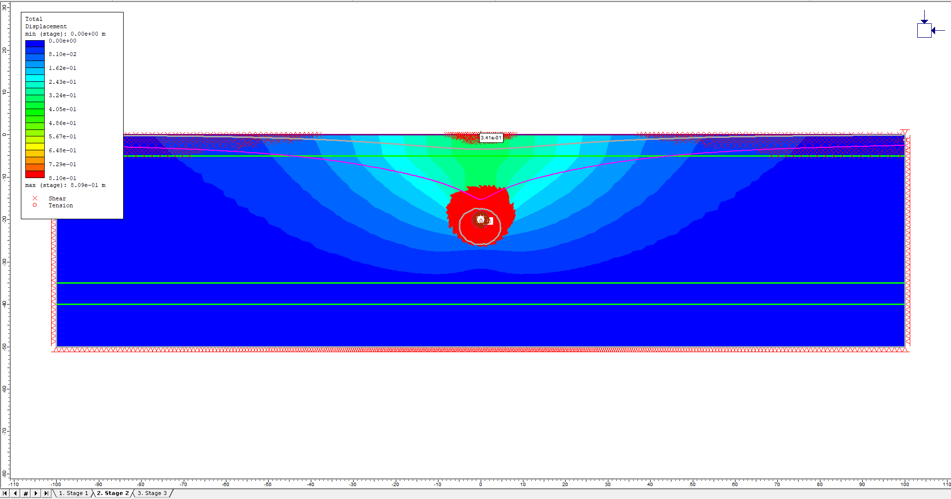
Turn off the Flow Vectors. Change the plot to show Total Displacement contours. Zoom out until you can see the ground surface. Click the button to Display Deformed Boundaries. Click the button to Display Yielded Elements. The plot should look like this:
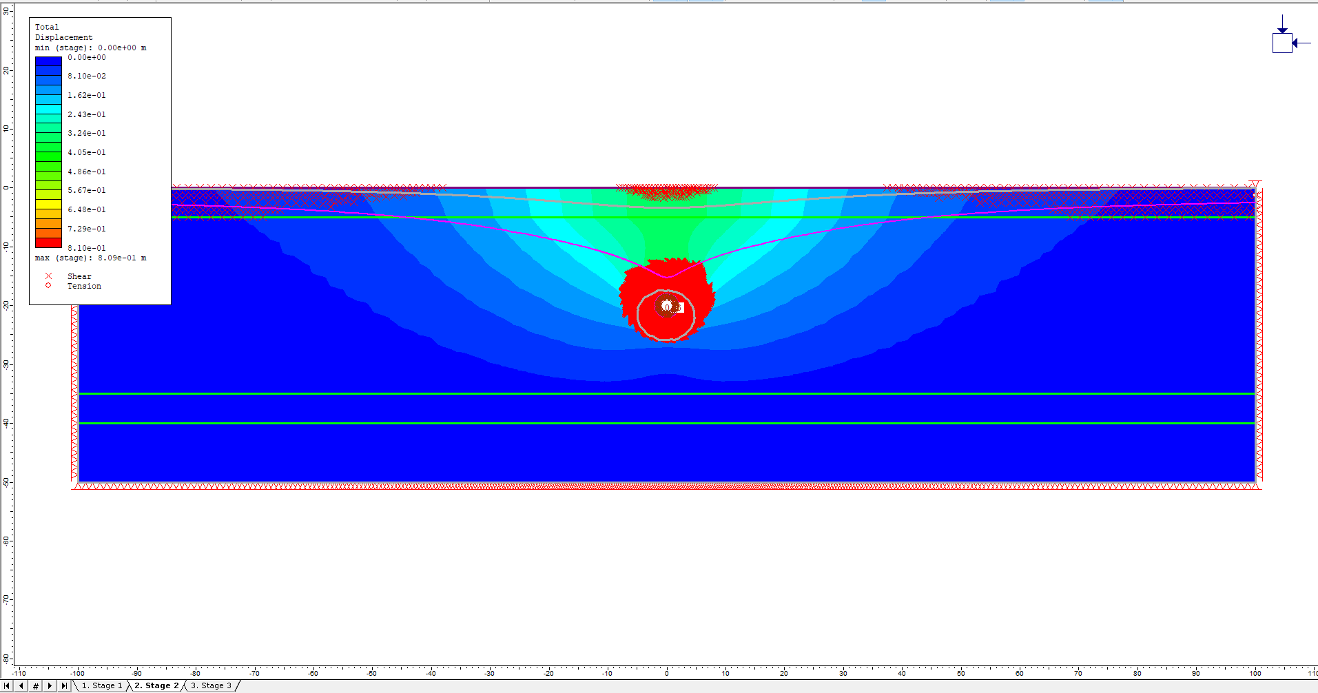
There is some shear failure visible around the tunnel and at the ground surface. There is also some subsidence at the surface. To determine the exact value, Select: Query > Add Material Query. Enter (0,0) for the query point and press Enter. In the resulting dialog, choose At Each Vertex and Show Queried Values.
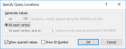
Click OK. The displacement directly above the tunnel will now be visible on the model.
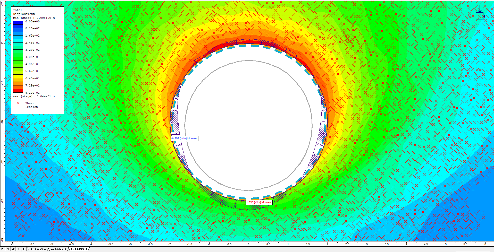
Select the Stage 3 tab. There is little change in the displacement or failure pattern (there is actually a small amount of rebound since removing the load is equivalent to removing material inside the tunnel).
The liner has successfully accommodated the load without any more failure. To evaluate the performance of the liner, ensure Stage 3 is selected, right-click on the liner, select Hide Water Table, right-click on the liner again and Select Show Values > Show Values Options to display the Show Values dialog. Check the box for Liners and choose Bending Moment from the pull-down menu.
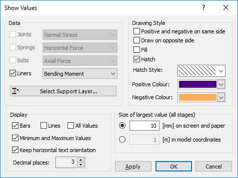
Click OK. Zoom in on the tunnel to see the moments as shown.
Finally, check the volume loss due to the tunnel excavation. The volume loss is the volume change due to surface subsidence divided by the volume of the excavation. Go to Analysis > Report Generator. Scroll down to the heading for Stage 3.
This concludes the Drawdown Analysis for Tunnel Excavation tutorial.
5.0 References
Shin, J.H., Addenbrooke, T.I. and Potts, D.M., 2002. A numerical study of the effect of groundwater movement on long-term tunnel behaviour. Géotechnique, 52 (6), 391-403.