Dynamic Data Analysis

1.0 Introduction

This tutorial starts from introducing the newest features in RS2 Dynamic Data Analysis. In this tutorial, an embankment is subjected to a dynamic loading at the base. The model consists of two soil layers and four stages and groundwater analysis is involved. In the starting model file, project settings, geometry and field stress have been defined. The tutorial will proceed from defining and assigning material properties. The dynamic data filter feature is incorporated in the model simulation. The focus of this tutorial is to compare the pore pressure build-up under seismic waves using two different material models: Finn and Mohr-Coulomb.

1. Select Files > Recent Folders > Tutorials Folder
2. Open the Load Input Filter tutorial file in the Dynamic Data Analysis tutorials folder.

2.0 Dynamic Data Analysis

1. Select: Dynamic > Dynamic Data Analysis

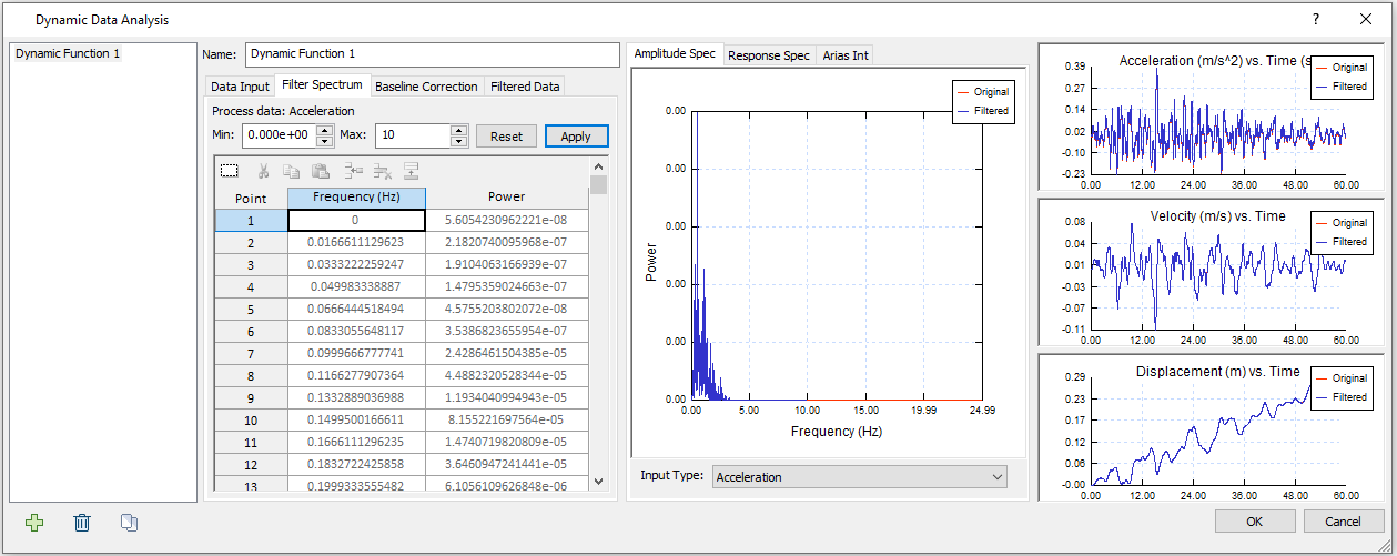
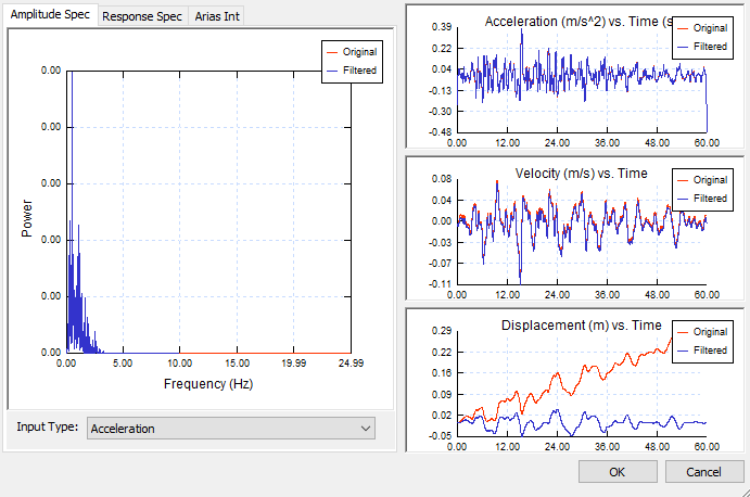
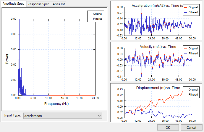
Once the load function time histories are entered, amplitude spectrum, time-acceleration, time-velocity and time-displacement graphs are plotted based on the input data. It can be selected that either the amplitude spectrum is generated based on acceleration or velocity.

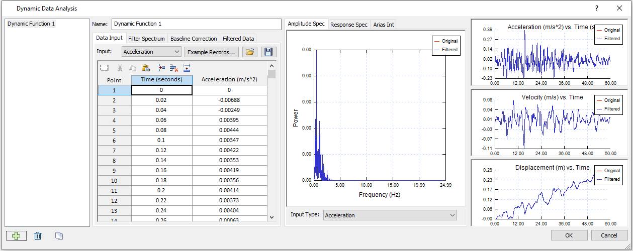
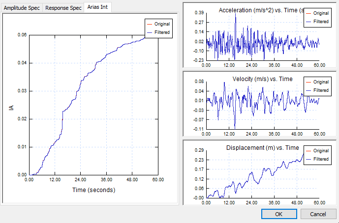
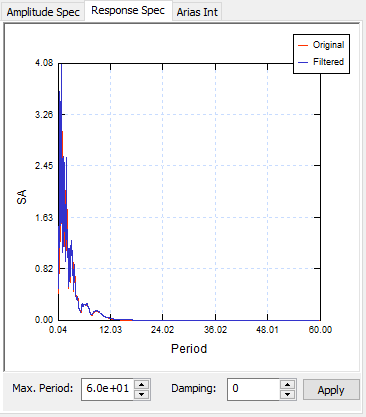
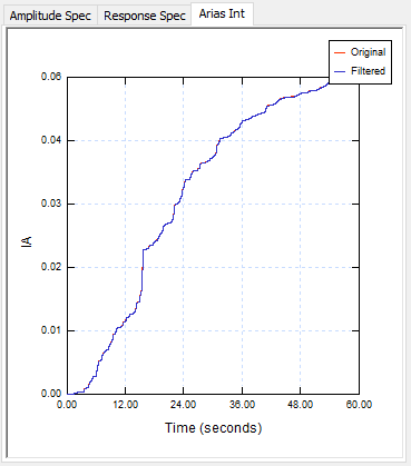
Response spectrum and arias intensity are also automatically plotted.

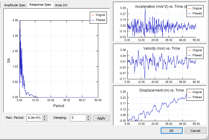
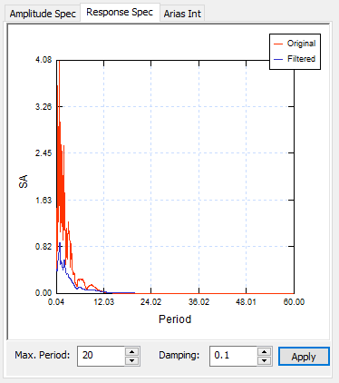
2.1 Response Spectrum

1. Select: Response Spectrum from the left graph.

The maximum period and damping ratio can be adjusted to compare with the original response spectrum.

2.2 Filter Spectrum

1. Select: Filter Spectrum, second tab from the data.

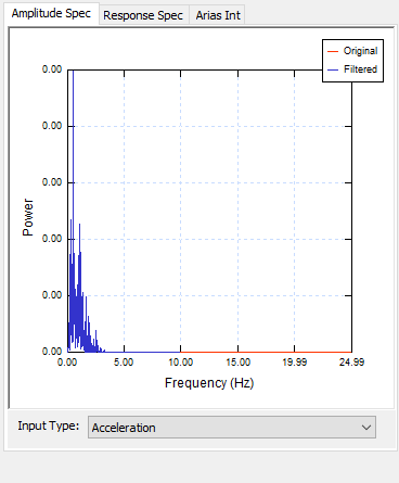
The minimum and maximum frequencies can be adjusted for filtering. As they are adjusted, all graphs are also replotted based on the filtered data set. Both the original and filtered dataset are plotted on all graphs for easy comparison. To find the global minimum and maximum frequencies of the entire data set, select to reset the Min and Max.

It can be observed from the Amplitude Spectrum that the amplitude is very minimal for frequencies bigger than 10, therefore, we set maximum frequency to 10 for the filter spectrum.

2.3 Baseline Correction

1. Select: Baseline Correction, third tab from the data.

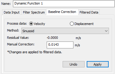
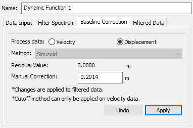
Two methods are available for baseline correction: Cut Off and Sinusoid. Both methods can be applied to velocity to correct the velocity drift. However, only Sinusoid method can be applied to displacement to correct the displacement drift. Once either velocity or displacement is corrected, new sets of acceleration and displacement or acceleration and velocity are calculated based on the corrected values and plotted on the graphs to compare with the original dataset. Please note that the baseline correction is applied to the original data, not the filtered data from Filter Spectrum.

For Cut Off method, an Applicable Cut Off Range is generated based on velocity data set, giving the users a reference on the range of Cut off value that outputs the optimal baseline correction. Click Apply to process the Cut Off. The Undo button is also available for users to take a step back.

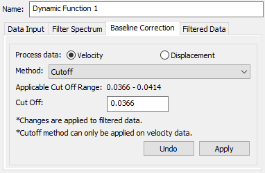
Similarly, a default value for the Sinusoid method, which is taken as the displacement/velocity value at the final timestep, is generated based on either velocity or displacement data set as a reference for the users. After clicking Apply, the residual value changed to 0, which means the baseline has been corrected.

3.0 Defining Material Properties

1. Select: File > Recent Folders > Tutorial Folder
2. In the Dynamic Analysis > Dynamic Data Analysis folder, open MC and Rayleigh (Initial).fez

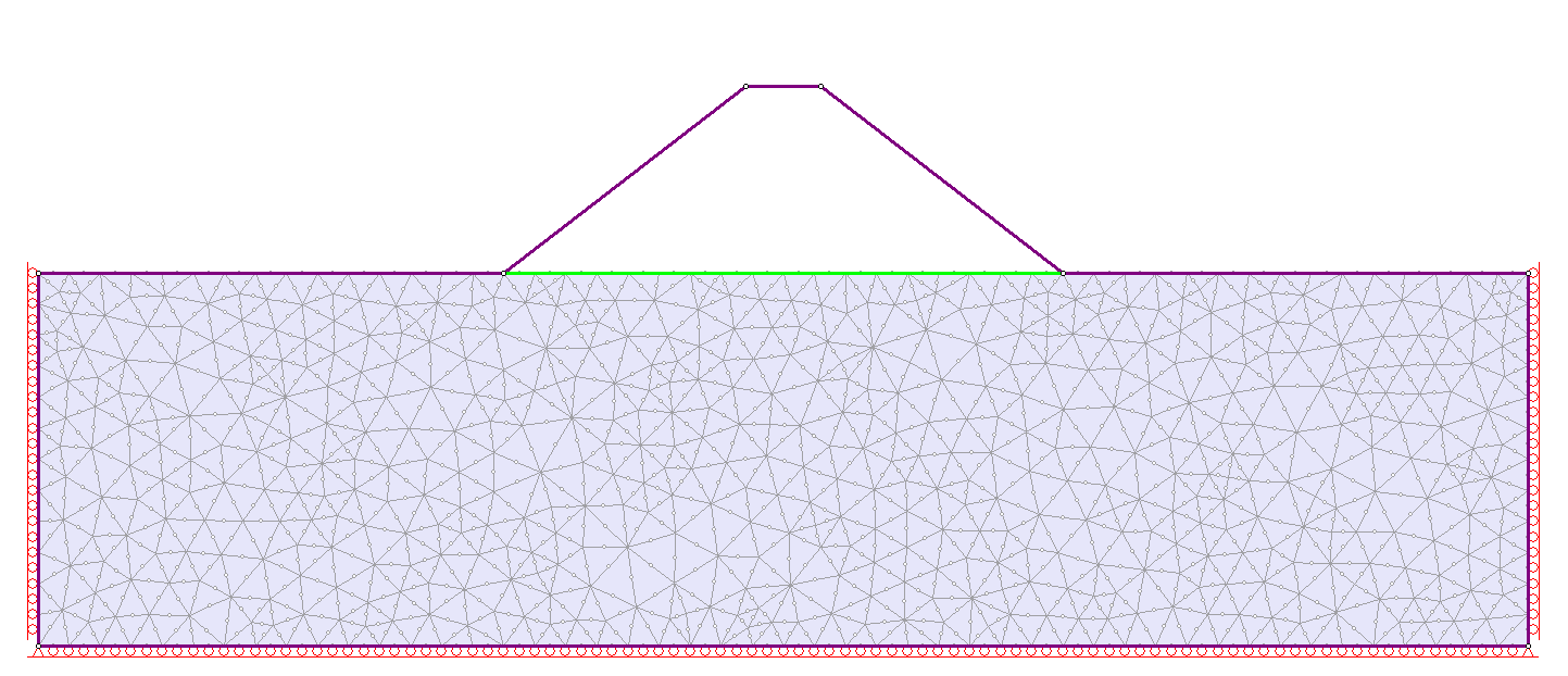
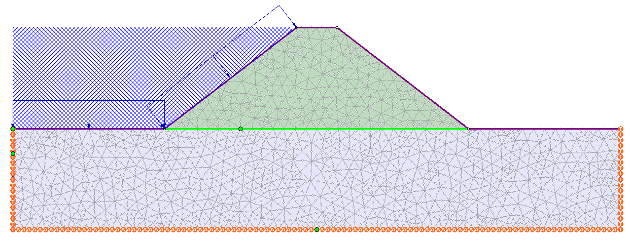
This file has the project setting, model geometry, boundaries, field stress, mesh, and restraints created. This tutorial will proceed to define material properties, determine groundwater conditions, set up dynamic boundary conditions, filter and apply the dynamic loading. Natural frequencies will then be computed to obtain the Rayleigh Damping parameters and apply to the project settings.

3.1 Material Properties

The only difference between the models using Finn model and Mohr-Coulomb model is the material properties, everything else is identical. Two material layers are used in this tutorial. This tutorial will start from the Mohr-Coulomb model.

1. Select: Properties > Define Material
2. Enter material properties for the Mohr-Coulomb model as follows.

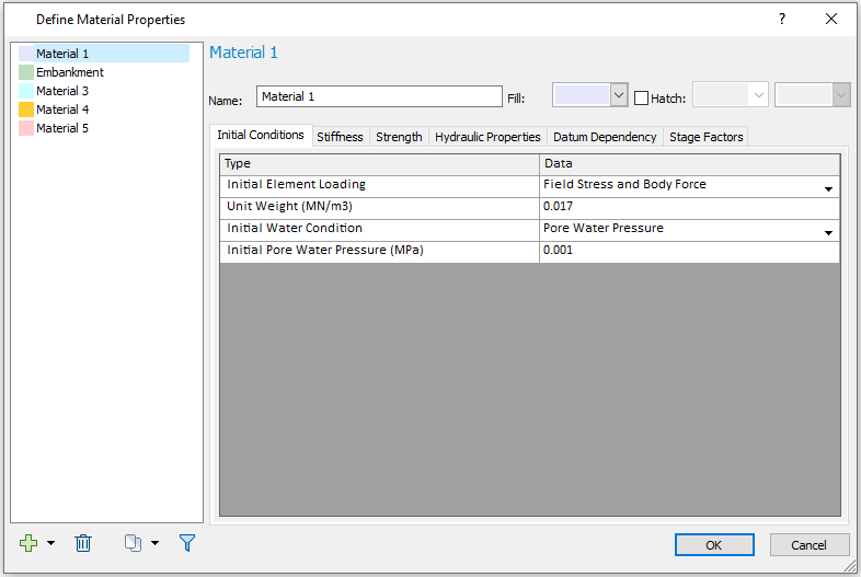
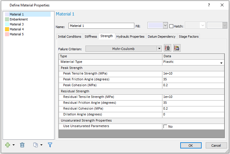
MATERIAL 1

Initial Conditions

Strength Parameters

Stiffness

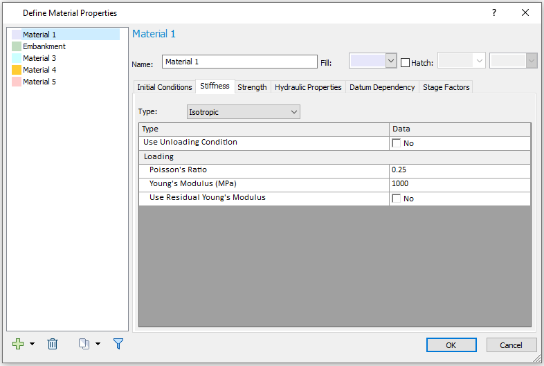
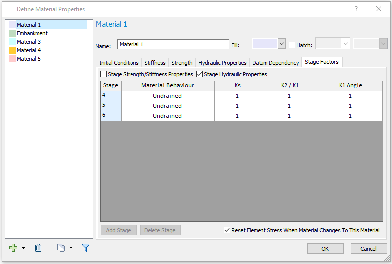
Stage Factors

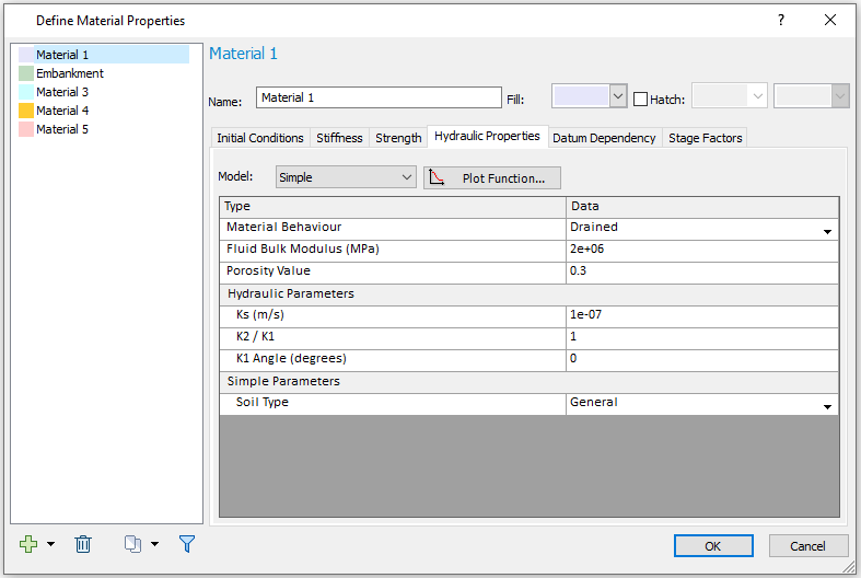
Hydraulic Properties

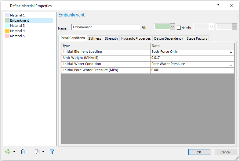
EMBANKMENT

For the embankment material, only initial conditions, stiffness and strength are different as shown in the following screenshots, the hydraulic properties, datum dependency and stage factors remain the same as material 1.

Initial Conditions

For Initial Conditions, the Initial Element Loading = Body Force Only:

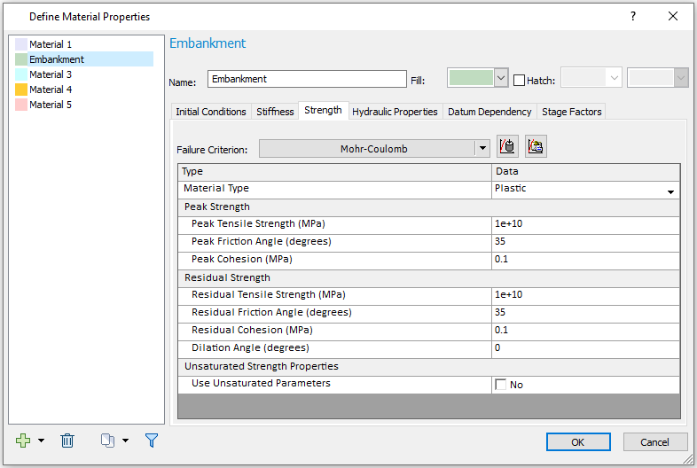
Strength

For Strength, Residual Cohesion (MPa) = 0.1:

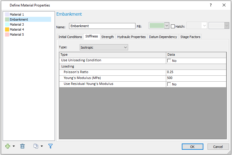
Stiffness

For Stiffness, the Young’s Modulus (MPa) = 500:

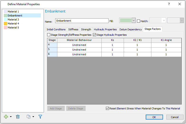
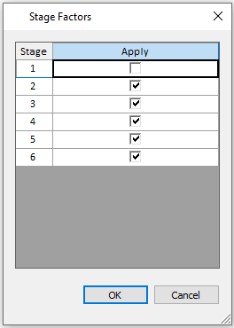
Stage Factors

Stage Factors for Embankment is the same as Material 1:

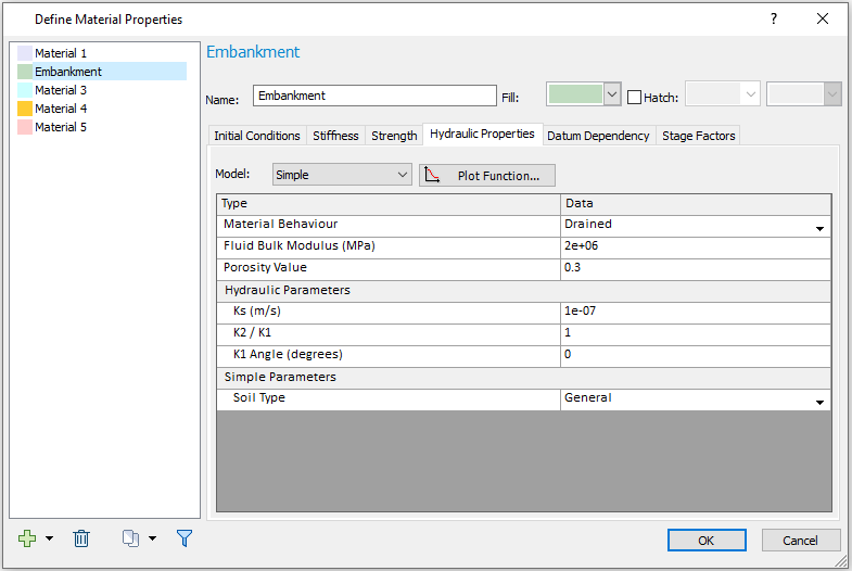
Hydraulic Properties

Hydraulic Properties for Embankment is the same as Material 1:

Select OK to save and close the Define Material Properties dialog.

3.2 Assign Material Properties

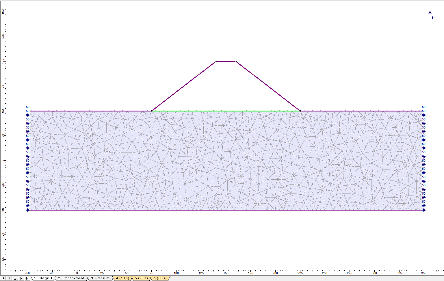
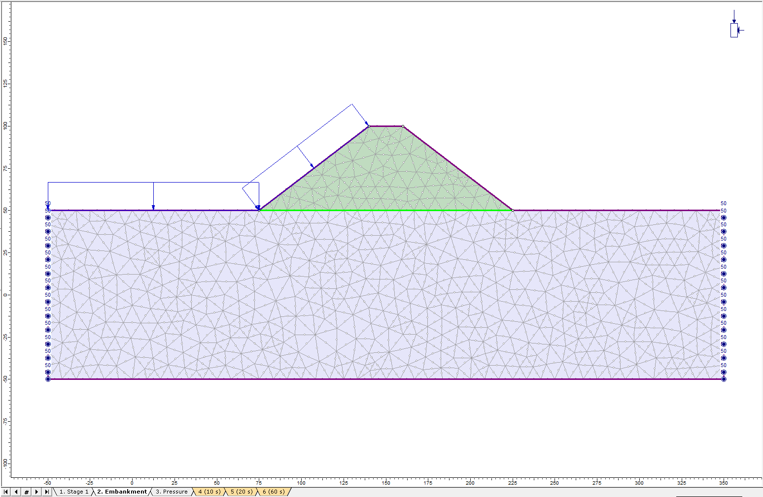
Click through all stages, ensure in Stage 1, Material 1 is assigned to the bottom layer while the top layer is excavated. From Stage 2 to 6, Material 1 is assigned to the bottom layer, and Embankment to the top layer.

4.0 Assigning Groundwater Conditions

Make sure the Groundwater workflow tab is selected throughout this section.

4.1 Set Boundary Conditions

1. Select: Groundwater > Set Boundary Conditions
2. Set BC Type to Total Head and input a Total head value of 50m.
   
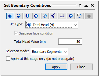
3. Make sure Stage 1 is selected.
4. Assign this boundary condition to the left and right sides at stage 1 as the follows:
   
5. Click Close to exit the Set Boundary Condition dialog.
6. Select Stage 3 (Pressure), right click at the left side. Select Remove Boundary Condition as the follows:
   
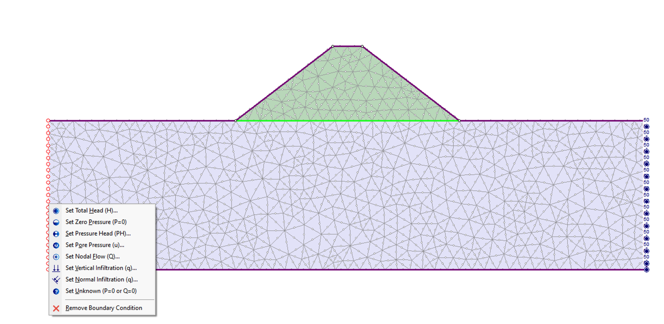
7. Repeat the same to the right side. Now the 50 m total head boundary condition should be applied only at stage 1 and 2 and removed at stage 3 to 6.
   
8. Select: Groundwater > Set Boundary Conditions
9. Set BC Type to Total Head and input a Total head value of 100m.
   
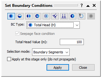
10. Make sure Stage 3 (Pressure) is selected. Assign this boundary condition to the left boundary of embankment, and top left boundary of Material 1 as the follows:
    
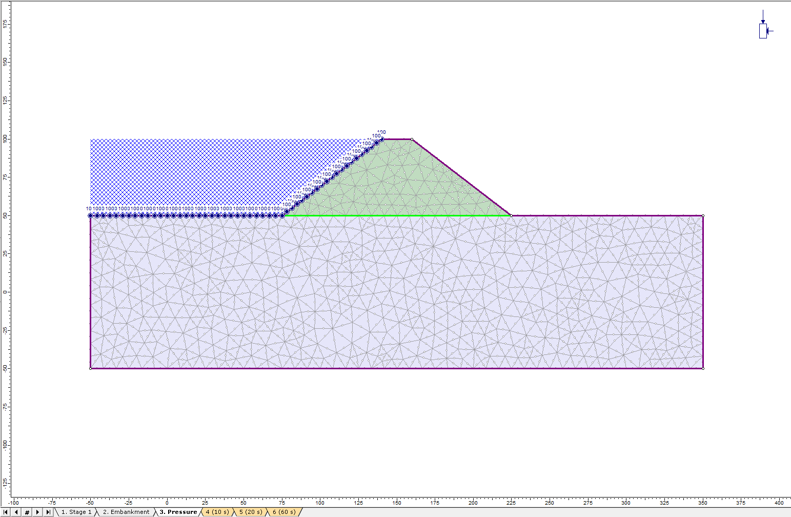
    Click through stages, now the 100 m total head should be applied to stages 3 to 6.
11. In the Set Boundary Conditions dialog, set BC Type to Unknown (P=0 or Q=0) and select Apply at this stage only (do not propagate).
    
12. Make sure Stage 3 (Pressure) is selected. Assign this boundary condition to the top and right boundary of the embankment, and the right top boundary of Material 1 as the follows:
    
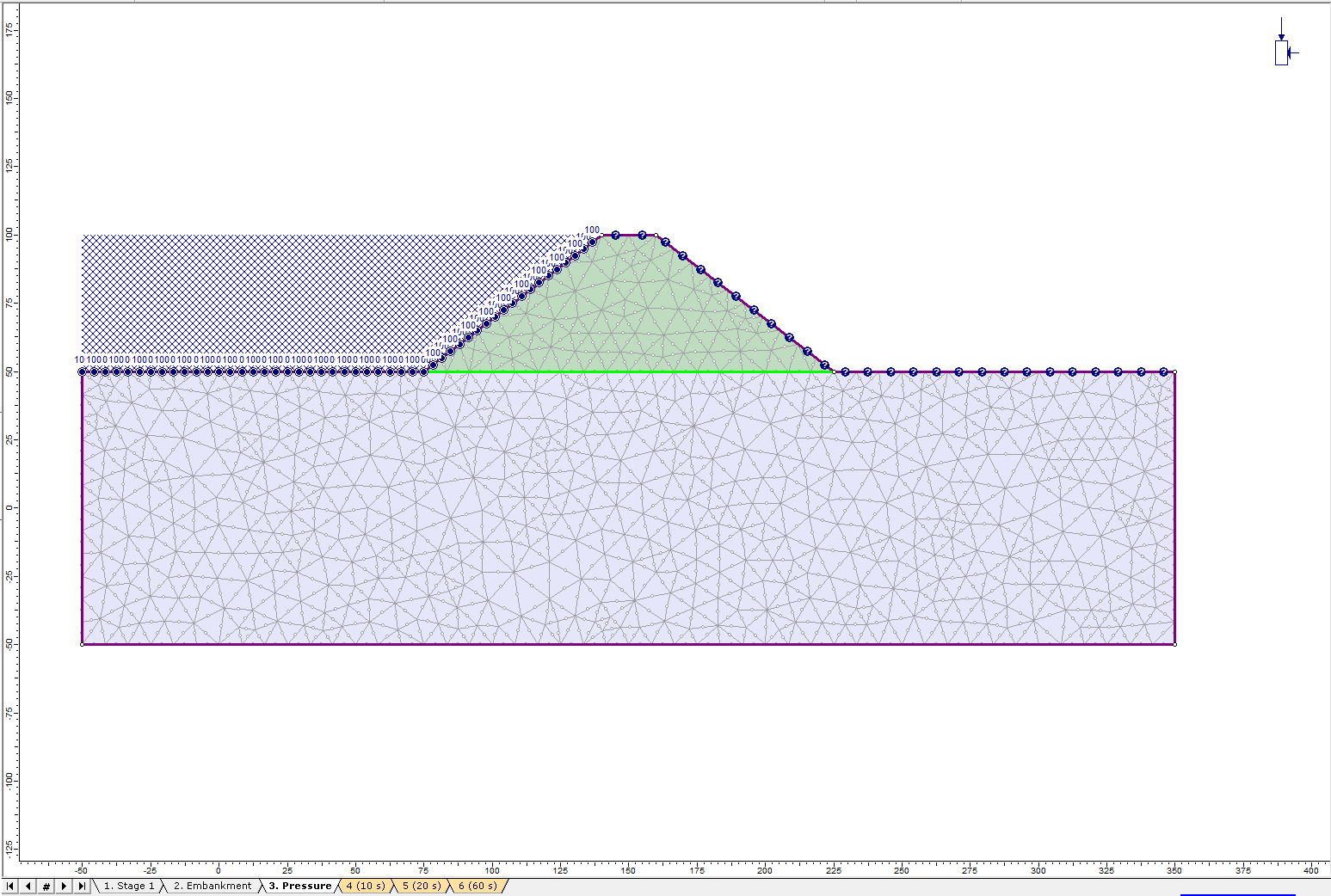
    Click through all stages, now the unknown boundary condition should apply only to stage 3.
13. In the Set Boundary Conditions dialog, set BC Type to Zero Pressure (P=0) and Selection mode to Boundary Nodes as the follows:
    
14. Make sure stage 4 (10 s) is selected. Click and hold the left mouse button, and drag a selection window which encloses a portion of top right boundary at the ground surface. Hit Enter or click Apply to assign the Zero Pressure boundary condition to the selected boundary nodes as the follows:
    
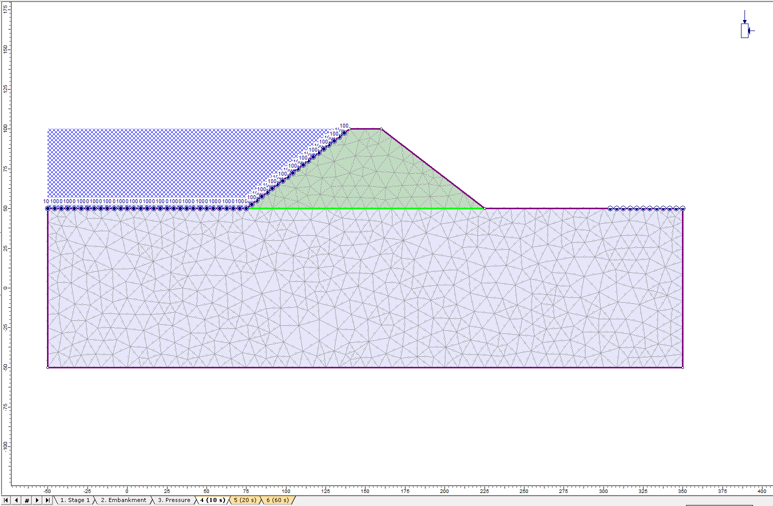
    Click through stages, now the Zero Pressure boundary condition should be applied to stage 4 – 6.
15. Click Close to exit the Set Boundary Conditions dialog.
    

4.2 Add Ponded Water Loads

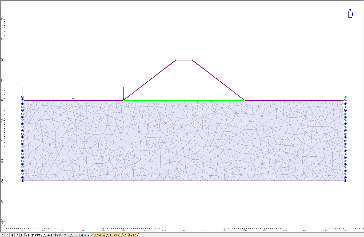
Make sure Stage 1 is selected.

1. Select: Loading > Ponded Water Loads > Add Ponded Water Loads
2. For Ponded Water Load 1, select the Use Calculated Water Pressure option as shown below:
   
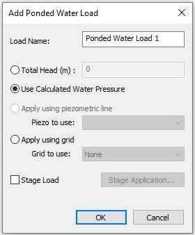
3. Click OK.
4. Enter coordinate (-50, 50) as the first point, and (75, 50) as the second point. Hit Enter to complete selection. Ponded Water Load 1 will be added to the boundary as the follows:
   
   
5. Select Stage 2.
6. Select: Loading > Ponded Water Loads > Add Ponded Water Loads
7. For Ponded Water Load 2, select the Use Calculated Water Pressure option. Check the Stage Load checkbox as shown below:
   
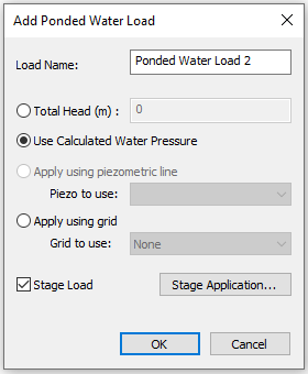
8. Click the Stage Application button. Check the Apply option for stages 2 to 6 as the follows:
   
   
9. Click OK to close both the Stage Factors dialog and the Add Ponded Water Load dialog.
10. Enter coordinate (75, 50) as the first point, and (140, 100) as the second point. Hit Enter to complete selection. Ponded Water Load 2 will be added to the sloped boundary as follows:

Click through all stages. Ponded Water Load 1 should be applied to all stages, and Ponded Water Load 2 to Stages 2 - 6.

5.0 Assigning Dynamic Conditions

5.1 Dynamic Data Analysis

In this tutorial, we use the seismic acceleration data from the 1985 Mexico City Earthquake. The data can be found in the Excel Sheet in the installation folder.

C:\Users\Public\Documents\Rocscience\RS2 Examples\tutorials\Dynamic Analysis\Dynamic Slope Analysis

1. Open the Excel file titled “Mexico City 1985 - Mesa Bivradora C. U.”
2. Ensure the first sheet, titled “Mexico City 1985” is selected.
3. Select: Dynamic > Dynamic Data Analysis
4. For Dynamic Function 1, under Data Input tab, select Input = Acceleration.
5. Copy and paste the time and acceleration data from Excel Sheet, sheet 1 “Mexico City 1985” (Column A and B) to the data grid as shown below:
   
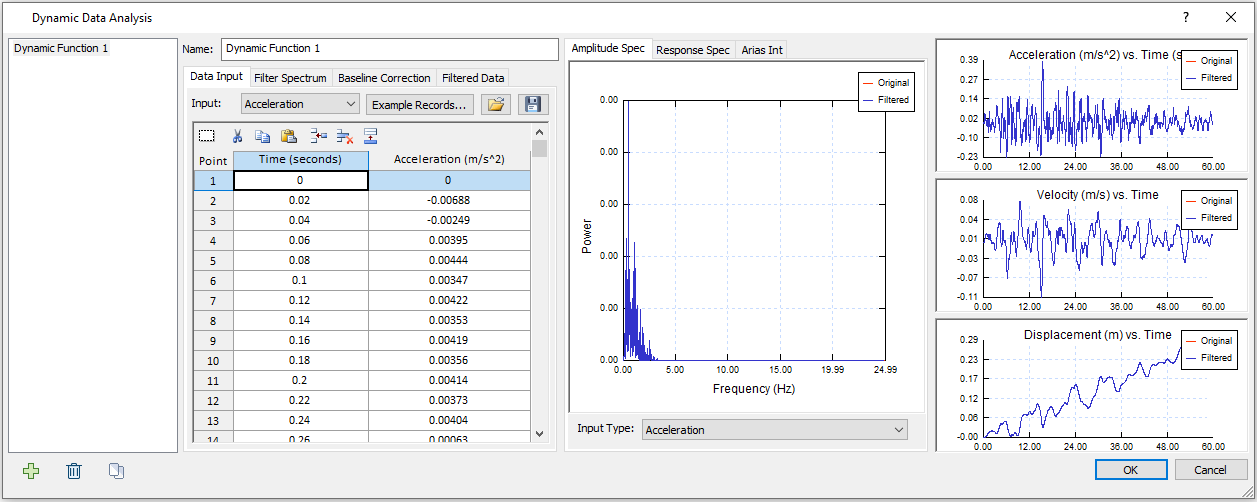
6. In the middle section of the dialog, make sure Input Type = Acceleration for the Amplitude Spec tab.
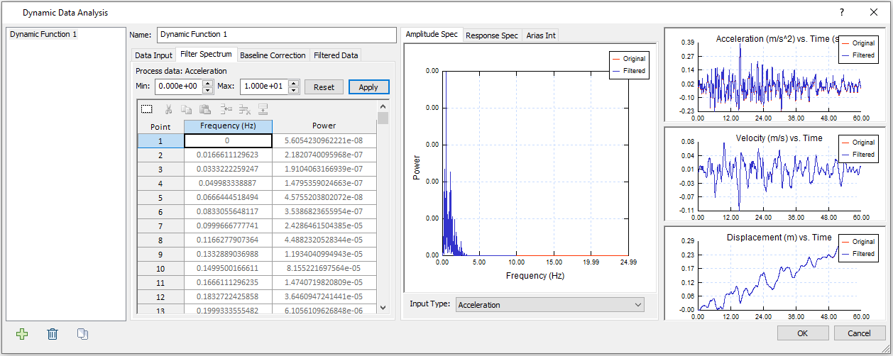
7. Select the Filter Spectrum tab.
8. As observed from the Amplitude Spectrum, little amplitude occurs beyond 10 Hz frequency. Thus, we can set Max = 10 and click Apply. Your dialog should look as shown below:
   
9. Select the Baseline Correction tab.
10. Choose Process data = Displacement, and the Method will be set to Sinusoid. By default, Residual Value = 0.2914 m, and Manual Correction is set to the same.
    
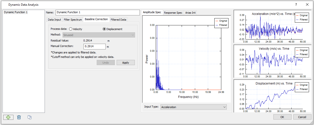
11. Click Apply to apply a Manual Correction of 0.2914 m. The dialog will display as shown:
    
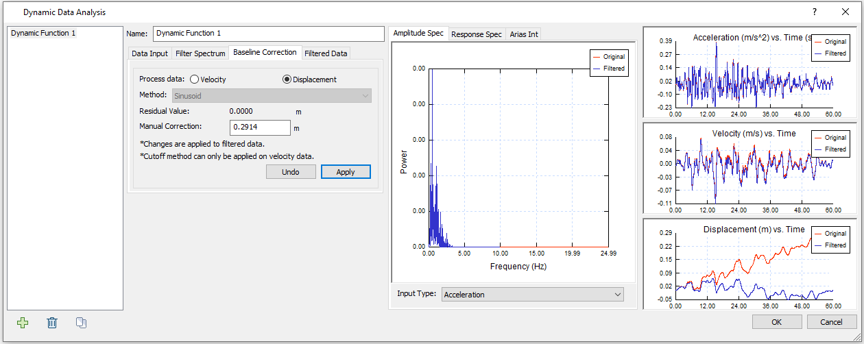
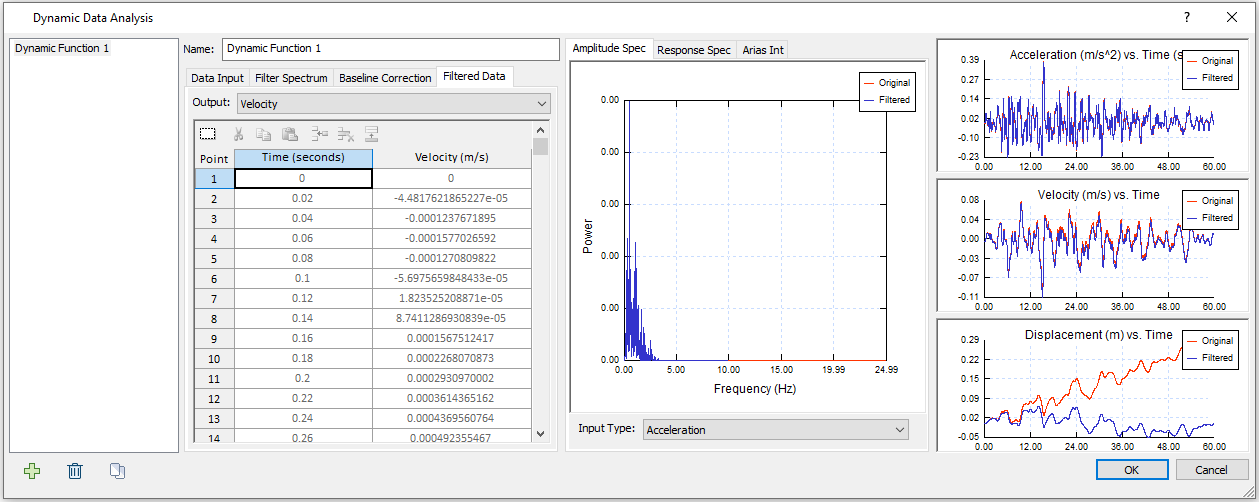
    Now the Residual Value has changed to 0 m. The change is not significant on Acceleration (m/s^2) vs. Time (s) or Velocity (m/s) vs. Time plots, but it is noticeable on Displacement (m) vs. Time plot.
12. Select the Filtered Data tab.
    

Output data type can be selected from the dropdown bar. We will use Velocity output as the dynamic load input for the next step.

5.2 Define Dynamic Loads

1. Select: Dynamic > Define Dynamic Loads
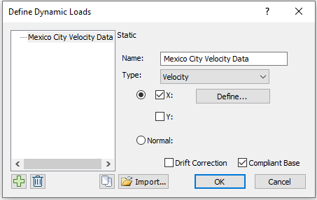
2. Rename “Dynamic Load 1” to “Mexico City Velocity Data”. Select Type = Velocity. Check the Compliant Base checkbox. Your dialog should look as follows:
   
3. Click the Define button.
4. In the Velocity vs. Time dialog, check the “Use filtered data” option at the bottom, and select Dynamic Function 1. The filtered velocity data earlier in Dynamic Data Analysis should be inputted as shown below:
   
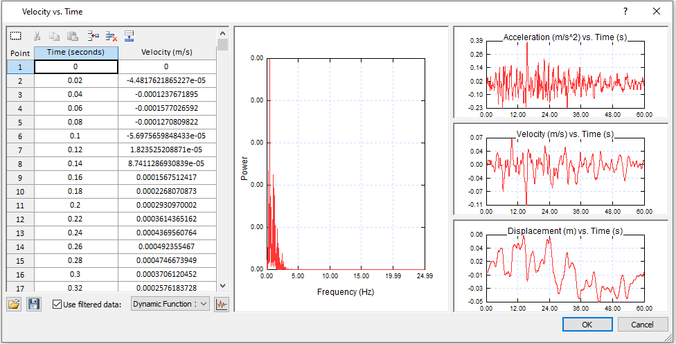
5. Click OK in both the Velocity vs. Time and Define Dynamic Loads dialogs.
   

5.3 Set Dynamic Boundary Conditions

1. Go to tab Stage 4 (the dynamic stage), and select Dynamic > Set Dynamic Boundary Conditions
2. Select BC Type > Absorb for the bottom boundary and select Transmit for the boundaries on the sides:
   
3. Click Close to exit the Set Dynamic BCs dialog. Now the dynamic boundary conditions should be applied to stage 4 - 6.
   

5.4 Assign Dynamic Load

1. Select: Dynamic > Add Dynamic Load…
2. Select Load Function = Mexico City Velocity Data (Velocity) and set Installed at stage to 4 as follows:
   
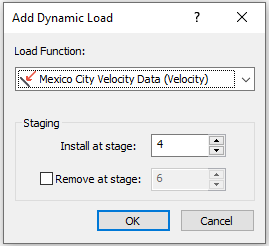
3. Click OK to close the dialog.
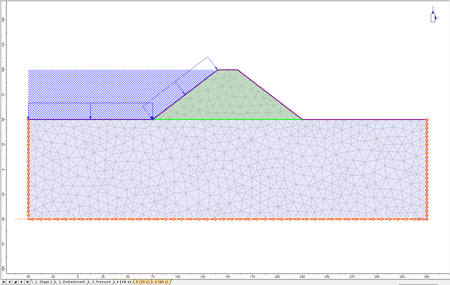
4. Use the selection tool to select the bottom boundary. Press Enter to complete selection. The Dynamic Load will apply as follows:

5.5 Define Rayleigh Damping

To decide the Rayleigh Damping parameters, we need to compute natural frequency based on the filtered velocity.

1. Select: Dynamic > Compute Natural Frequencies…
2. Enter Minimum Frequency = 1e-05 Hz and Maximum Frequency = 20 Hz. Then click Compute…
   
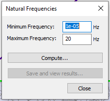
3. Once the computation is done, select save and view results. The Natural Frequencies Results – Rayleigh Damping dialog should look as follows:
   

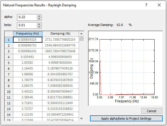
The fourth and fifth frequency numbers on the table (0.535 Hz and 1.054 Hz) need to be inputted in project settings in the next step.

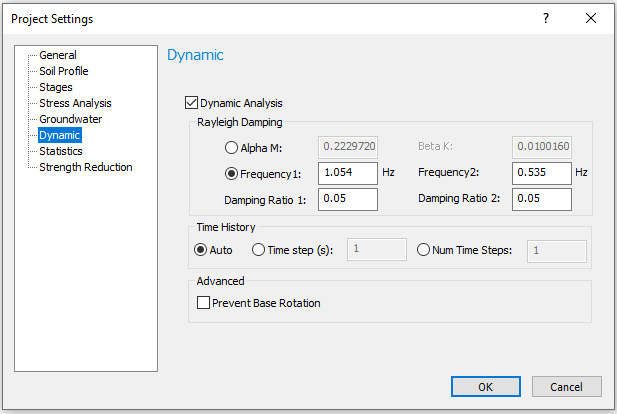
4. Select: Analysis > Project Settings and go to the Dynamic tab.
5. Under Rayleigh Damping, select the second option.
6. Enter:
• Frequency 1 = 1.054, Frequency 2 = 0.535
• Damping Ratio 1 = 0.05, and Damping Ratio 2 = 0.05.

Now the defined dynamic analysis parameters are inputted. Your dialog should look as follows:



7. Click OK.

5.6 Add Time Queries

1. Select: Dynamic > Time Query > Add Solid Time History Query
2. Enter the coordinates (113, 50). Hit Enter to add the point and hit Enter again to complete selection. Now a time query point on the material boundary between Embankment and Material 1 has been added.

This step concludes the completion of the Mohr-Coulomb model construction.

3. Save the model as “MC and Rayleigh.fez”.

6.0 Change to Finn Model

To compare the results between Mohr-Coulomb and Finn model, save the model we just created as a separate file, “Finn and Rayleigh.fez”. In this new saved Finn model, change the material properties as following:

1. Select: Properties > Define Materials
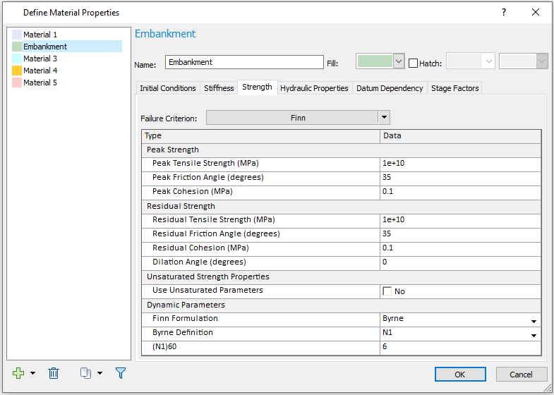
2. For Material 1, under the Strength tab, change Failure Criterion to Dynamic > Finn. Under the Dynamic Parameters section, select Finn Formulation = Byrne, Byrne Definition = N1, and (N1)60 = 10.
3. For Embankment, under the Strength tab, change Failure Criterion to Dynamic > Finn. Under the Dynamic Parameters section, select Finn Formulation = Byrne, Byrne Definition = N1, and (N1)60 = 6.
   
   The initial conditions, hydraulic properties, datum dependency and stage factors remain the same as the Mohr-Coulomb model. Your dialog should look as follows: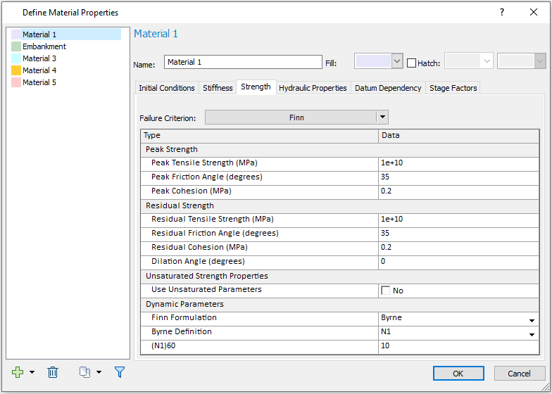
   
   
   
4. Click OK to close the dialog.
   
   Other settings remain unchanged. Now, we are ready to run analysis for both models.
   
5. Select: Analysis > Compute
   

7.0 Results

When the models finish running, open Interpret to see the results.

1. Select: Analysis > Interpret
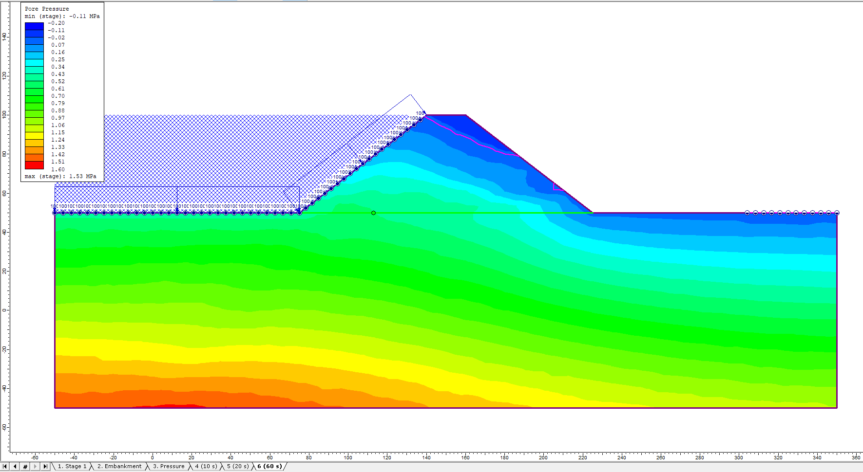
2. Click the tab for Stage 6 to observe the final pore pressure
3. Change the contours to plot pore pressure using the drop-down menu in the toolbar.

7.1 Pore Pressure Contour

MOHR-COULOMB MODEL

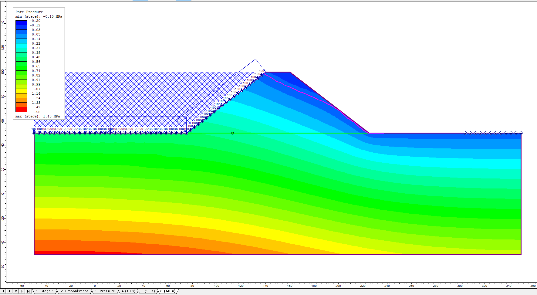
FINN MODEL

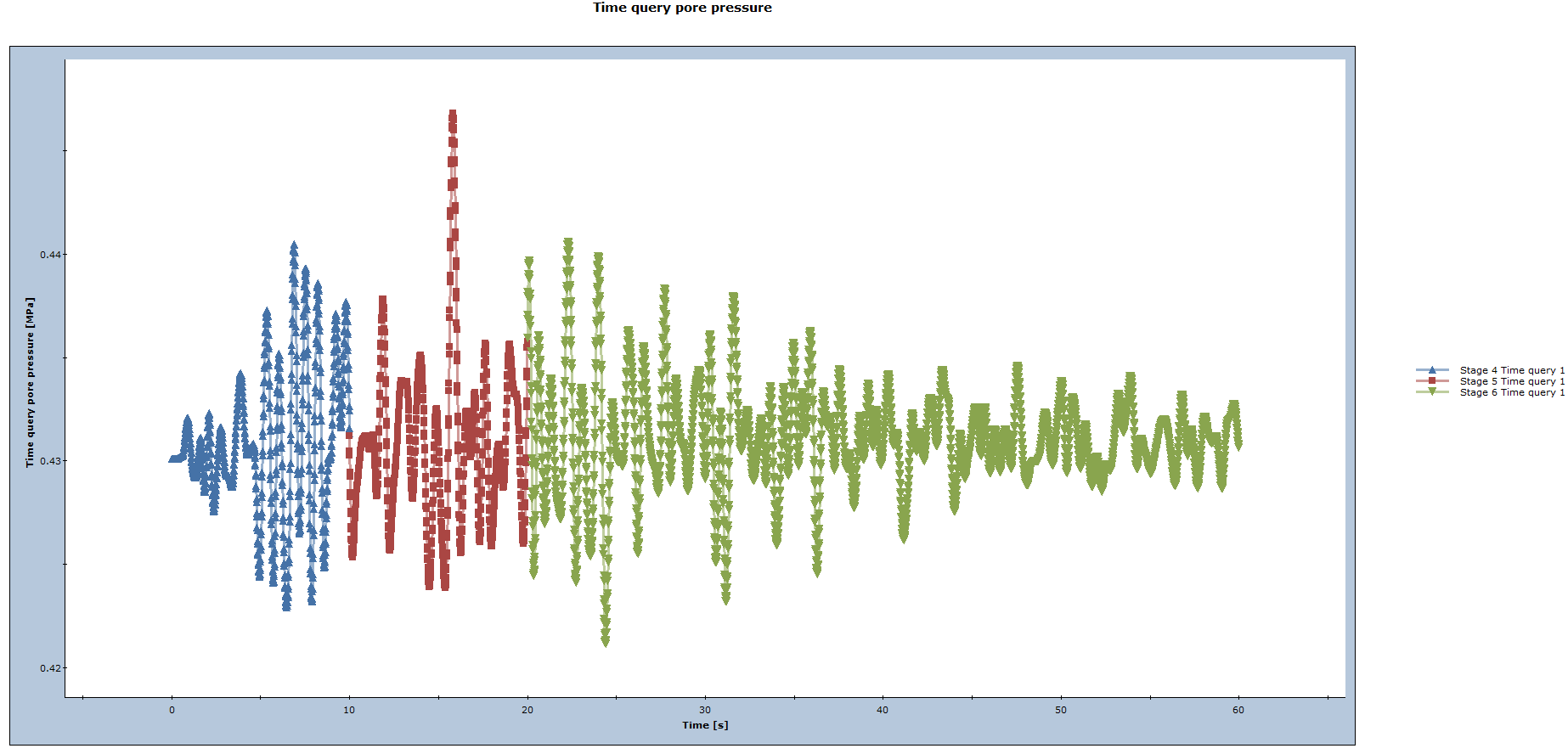
7.2 Pore Pressure Graphs at Time Query

Right click the time query and select pore pressure in the menu to plot the pore pressure changes through all stages over time for both models.

MOHR-COULOMB MODEL

FINN MODEL

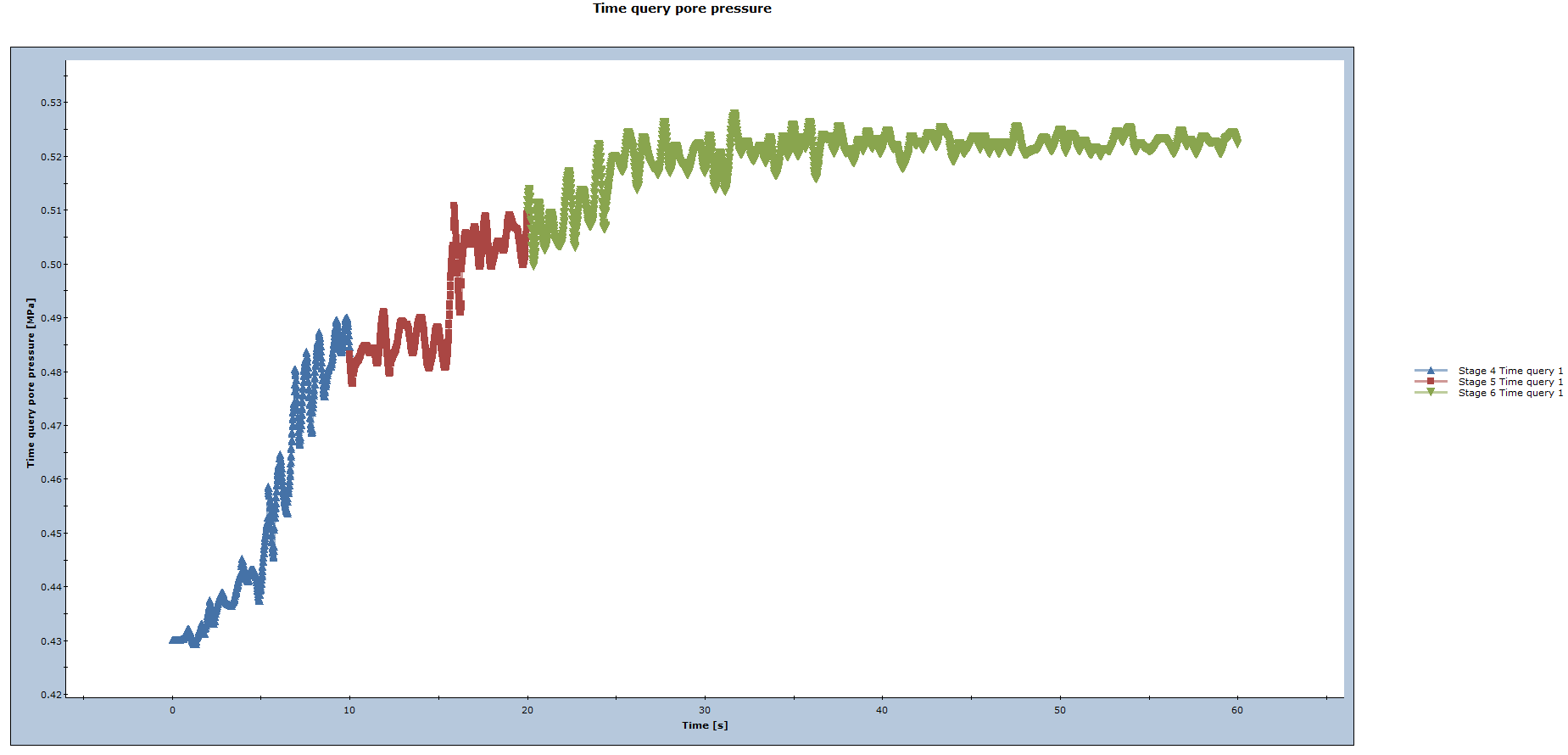
Notice that Finn model results in higher pore pressure at the end of the time period than the Mohr-Coulomb model.

This concludes the tutorial.