Dynamic Slope Analysis C

Rayleigh Damping

1.0 Introduction

Considering a dynamic system:

[K] is the linear stiffness matrix of the structure constructed with initial tangential stiffnesses. Thus, [C] consists of a mass-proportional term and a stiffness-proportional term.

The procedure to determine αM and βK involves choosing appropriate values of damping, to the degree possible, to the modes of linear system, which is represented by equation (1).

Damping of mode i is quantified by the damping ratio, ξi, the ratio of the mode’s damping to the critical value. If αM and βKare known, ξi can be calculated from:

Thus, αM and βK can be set to give any damping ratio to any two modes. The damping amount of other modes can also be computed from equation (2).

This procedure results in a nearly constant value of damping for modes with a frequency in the range from to R where R>1

In this tutorial, RS2 is used to determine the appropriate damping Rayleigh values for a model using the following steps:

1. Calculate the equilibrium state.
2. Apply dynamic conditions.
3. Run the undamped model
   
4. Determine the natural frequency range with power spectrum analysis.
5. Determine damping Rayleigh of the model.
6. Compare undamped and damped results.

2.0 Constructing the Model

2.1 Project Settings

1. Select: Analysis > Project Settings
2. Under the General page, define the units as being “Metric, stress as kPa”. For this tutorial, the Time Units need to be specified as "Seconds".
   
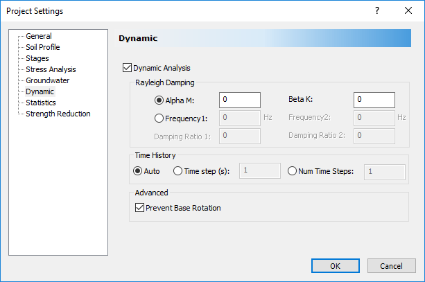
3. Select the Dynamic tab. Check the Dynamic Analysis check box to enable the dynamic analysis to be conducted on specific stages. On this tab, the general dynamic parameters are defined, such as Rayleigh Damping. Let’s start with an undamped model. Set Alpha M = 0, Beta K = 0.
4. The remaining parameters are left at their default values.
   
   In addition to an initial static stage, a dynamic stage will be added to see the final state of the model. The earthquake acceleration history has a duration of 60 seconds, but this tutorial only examines the intermediate stage after 55 seconds.
5. Select the Stages tab. The first stage in the analysis is, by default, always a static analysis stage. Insert a new stage and check the Dynamic check box. In the time column, the simulation time at which each stage will end is inserted. Change the time of the second stage to 55 seconds. Rename the second stage to “Intermediate 1.”
   
6. Select the Stress Analysis tab. Keep all parameters default as shown in the following dialog.
   
   The remaining parameters are left at their default values.
7. Close the Project Settings dialog by pressing the OK button.
   

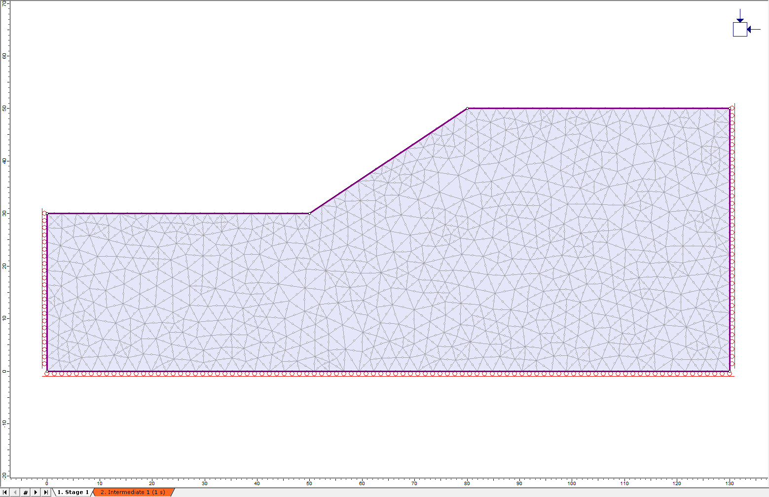
2.2 Boundaries

This model only requires an External boundary to define the geometry.

1. Select: Boundaries > Add External
2. Enter the following coordinates: (130, 0), (130, 50), (80, 50), (50, 30), (0, 30), (0, 0), and press “c” to close the boundary.

2.3 Material Properties

Define the material properties of the soil that comprises the slope.

1. Select: Properties > Define Materials
   This tutorial only uses one material.
2. Select the Initial Conditions tab.
• Change the material name to Till.
• Make sure the Initial Element Loading is set to Field Stress & Body Force (both in-situ stress and material self-weight are applied).
• Enter 19 kN/m3 for the Unit Weight.



3. Select the Stiffness tab.
• Enter 100 000 kPa for the Young’s Modulus and 0.4 for the Poisson ratio.



4. Select the Hydraulic Properties tab.
• Change the Static Water Mode to Ru.



5. Select the Strength tab, make sure the Failure Criterion is set to Mohr-Coulomb.
• Set the Material type to Elastic. Set the peak Tensile Strength and the peak Cohesion to 5 kPa.
• Set the peak Friction Angle to 38°.
• Keep “Use Unsaturated Parameters” unselected.



6. Press the OK button to save the properties and close the dialog

2.4 Field Stress

Define the in-situ stress field:

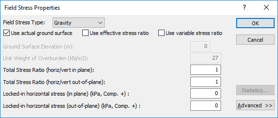
1. Select: Loading > Field Stress
2. Ensure the Field Stress Type is set to Gravity (gravitational stress distribution throughout the slope).
3. Check the Use actual ground surface check box. By using this option, the program will automatically determine the ground surface above every finite element and define the vertical stress in the element based on the weight of material above it.
4. Leave the horizontal stress ratios as 1, meaning hydrostatic initial stresses (i.e. horizontal stress = vertical stress). If the actual horizontal stress ratio is known, use this information. However, the horizontal stress distribution within a slope is rarely known, so leaving the default hydrostatic stress field has shown to be a good assumption. Select OK.

2.5 Mesh

Now, generate the finite element mesh. First, it's necessary to define the parameters (type of mesh, number of elements, type of element) used in the meshing process.

1. Select: Mesh > Mesh Setup
2. In the Mesh Setup dialog, change the Mesh Type to Uniform, the Element Type to 6 Noded Triangles, and the number of elements to 1500.
   
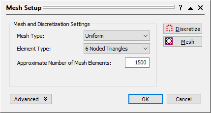
3. Close the Mesh Setup dialog by selecting the OK button.
4. Select: Mesh > Discretize and Mesh

2.6 Boundary Conditions (External)

The portion of the external boundary representing the ground surface (0,30 to 50,30 to 80,50 to 130,50) must be free to move in any direction.

1. Select: Displacements > Free
2. Use the mouse to select the three line segments defining the ground surface of the slope.
3. Right-click and select Done Selection.

For this analysis, the lateral boundaries will be allowed to move vertically and only be restrained in the horizontal direction in Stage 1. In Stage 2, all restraints will be removed.

4. Select: Displacements > Set Displacement
5. Enter Displacement in X direction = 1 and uncheck the Displacement in Y direction check box.
6. Check the “Stage displacements” box and click on the Stage Factors button. In the dialog, change the factor of Stage 1 to zero. Check the Free box for Stage 2.
   

A factor of zero represents a zero-displacement boundary condition. The free check box means that the nodes in Stage 2 are free to move without restraint. A factor of 1 means that the displacement will be equal to the magnitude(s) entered in the Nodal Displacement dialog.

Therefore, all lateral restraints were removed in the second stage and a zero-displacement boundary was set in the x-direction condition in Stage 1.

7. Select OK in the Stage Factors dialog and select OK in the Nodal Displacement dialog.
8. Using the resulting selection tool, click on the lateral boundaries and press Enter.

To free the bottom boundary:

9. Select: Displacements > Set Displacement
10. Enter Displacement in X direction = 1, Displacement in Y direction = 1.
11. Check the “Stage displacements” box and click on the Stage Factors button. In the dialog, change the factor of Stage 1 to zero. Check the Free box for Stage 2.
12. Select OK in the Stage Factors dialog and select OK in the Nodal Displacement dialog.
13. Using the resulting selection tool, click on the bottom boundary and press Enter.

In Stage 1, the displacement boundary conditions should appear as follows.

Now click on the Intermediate 1 tab at the bottom left of the window. Notice that Intermediate 1 has no restraints, as defined.

2.7 Boundary Conditions (dynamic)

Let’s assign dynamic boundary conditions to the boundaries of the model.

1. Ensure that the second stage of the Dynamic workflow tab is selected.
2. Right-click on one of the lateral sides of the model and select Set Transmit BC. Do this for both lateral sides of the column.
3. Right-click on the bottom boundary and select Set Absorb BC.
4. Save the model using the Save option in the File menu as Undamped Model.

2.8 Dynamic Load

Let’s input the earthquake data for the 1985 Mexico City earthquake as a dynamic load. This data can be found in Sheet 2 of the Excel Sheet in the installation folder. The file path is:

C:\Users\Public\Documents\Rocscience\RS2 Examples\tutorials\Dynamic Analysis\Dynamic Slope Analysis

1. Open the Excel file titled “Mexico City 1985 - Mesa Bivradora C. U.”
2. Select: Dynamic > Define Dynamic Loads
3. Rename “Dynamic Load 1” to “Mexico City Velocity Data.” Change the Type to Velocity and check the “Compliant Base” check box.
   
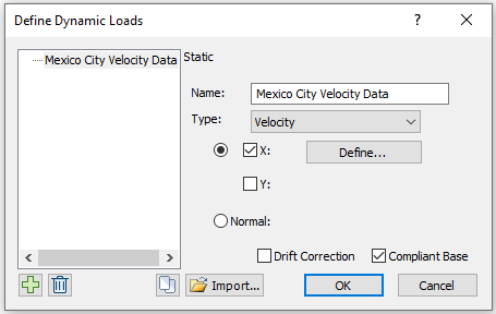
4. Click the Define button. Copy and paste the time data (Sheet 2, Column A) and the velocity data (Sheet 2, Column B) from the Excel sheet into the Velocity vs. Time dialog. The dialog should look as follows:
   
   
5. Click OK to save and close the Velocity vs. Time dialog. Click OK again to exit the Define Dynamic Loads dialog.
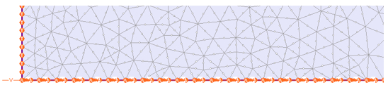
6. Select: Dynamic > Add Dynamic Load
7. In the resulting dialog, the Load Function should be the dynamic load previously defined and installed at stage 2. Click OK. Using the selection tool, click on the bottom boundary and press Enter.

The boundary should look as follows:

2.9 Time Query

Several time steps will occur between the defined stage times; RS2 will not output data for all the nodes for these intermediate time steps. However, the modeller does allow the user to specify time query points in the mesh. Time Queries records the dynamic data for all dynamic time steps occurring in the simulation. For this model, three time queries will be created.

1. Select: Dynamic > Add Solid Time History
2. Clicking anywhere in the slope will place a query at that point, or the exact coordinates may be typed in. Add time query points at the following locations on the slope: (80, 50), (80, 35), and (80, 20). Press Enter after each coordinate pair. Press Esc once all-time queries have been entered.

3.0 Results and Discussion

1. Select: Analysis > Compute
2. Select: Analysis > Interpret
3. Click on the Intermediate 1 tab at the bottom left of the window to view the results.
4. Right-click on the top-most time query point (80, 50) and select “Graph Time Query Data.” Set the Vertical Axis to “X Velocity” and the Horizontal Axis to “Time,” and click Plot.
5. Right-click on the plot and select “Plot in Excel.” On the Excel file, Sheet 1, copy the “Time [s]” and “Time query x velocity [m/s]”. We will use this output X Velocity data to analyze natural frequencies in the damped model.
6. Without closing Interpreter, return to the RS2 modeller.

Now start the damped model.

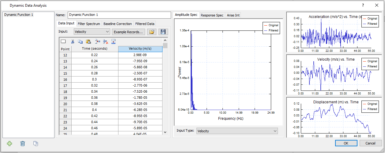
7. Select: Dynamic > Dynamic Data Analysis
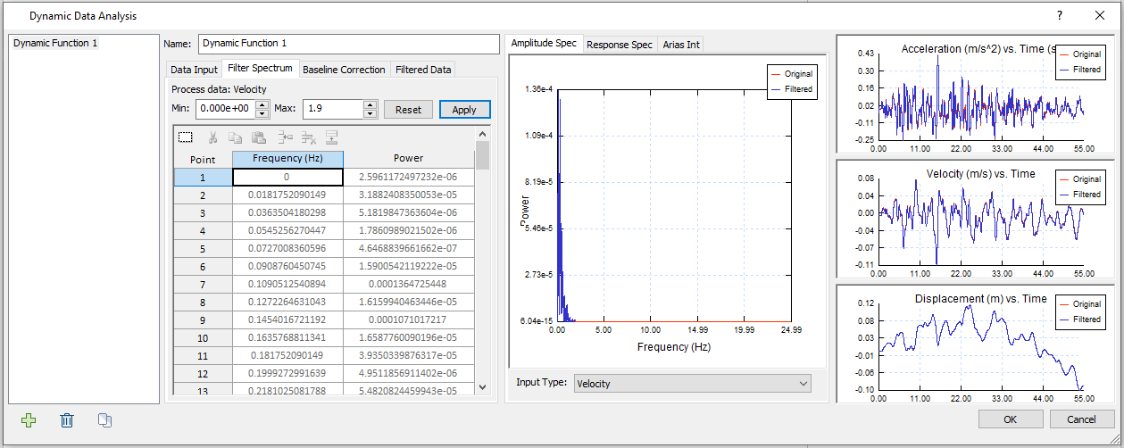
8. Select the Data Input tab under Dynamic Function 1, ensure the Input is Velocity.
9. For the first data point, manually enter Time (seconds) = 0, Velocity (m/s) = 0.
Note: The first data point in the data input grid must start at time = 0 s in the order for the power spectrum to handle the data properly.
10. From the second data point, paste the copied data from the undamped model result.
11. Make sure Input Type = Velocity under the Amplitude Spectrum tab, to show the “Power vs. Frequency (Hz)” plot base on velocity. The dialog should look as follows:
    
12. Select the Filter Spectrum tab. Enter a max value of 1.9 Hz and click the “Apply” button to the right. The two columns display the Frequency (Hz) vs. Power data within the defined range. Your dialog should look as follows:
    

Since most of the power occurs between 0 and 1.9 Hz, the power greater than 1.9 Hz can be filtered out. To further investigate the power distribution less than 1.9 Hz, the Power vs. Frequency (Hz) is plotted in Excel as shown below:

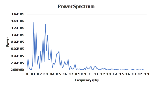
It can be observed that less power of the earthquake as toward 1.9 Hz, and the critical frequencies occur at around 0.1 Hz and 0.3 Hz, which are far from the 1.9 Hz boundary.

Similarly, for query point (80, 35) and query point (80, 20), the critical frequencies occur at approximately 0.1 Hz and 0.3 Hz.

Therefore, most of the important frequencies of the model occur under the 1.9 Hz mark. The damping Rayleighs in this case will be determined so that the average damping for all the natural frequencies from (0 Hz to 1.9 Hz) is 5%.

13. Click Cancel in the Dynamic Data Analysis dialog.
The purpose of this power spectrum analysis is to determine the natural frequency range, thus no need to save the filtered data.
14. Close Interpret and save the model.
15. Now select File > Save As and save the model as Damped Model.
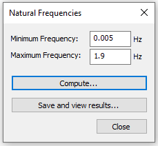
16. Select: Dynamic > Natural Frequencies > Compute Natural Frequencies.
17. Set the Min Frequency to 0.005 (to avoid extremely small, negligible values) and the Max Frequency to 1.9 Hz.
    
18. Select: Analysis > Compute
19. The computation may take several minutes. Once complete, select Save and View Results.

Notice that all the frequencies displayed fall in our range of 0.005 to 1.9 Hz.

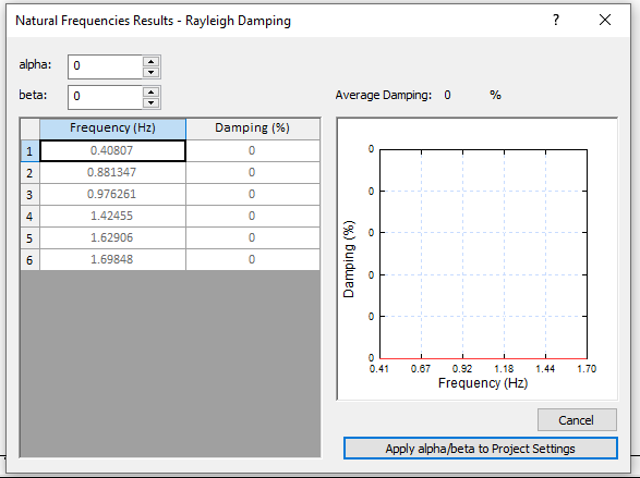
In the Results window, we want each individual damping value to be as close as possible to 5%. Manually adjusting the values of α_M and β_K may give the following values:

• α_M = 0.20
• β_K = 0.0089

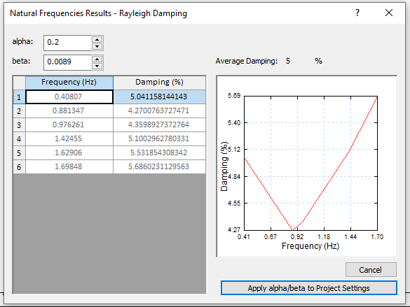
1. Click on “Apply alpha/beta to the Project Setting” to apply the parameters to the project.
2. Now, select Project Settings > Dynamic.

The Rayleigh Damping coefficients have been changed to Alpha M = 0.2 and Beta K = 0.0089.

It will be left as an exercise for the user to analyze the model with the new damping coefficients.

This concludes the Dynamic Slope Analysis Part C Tutorial.